Re-typing the data into the preferred layout takes time and is certain to result in errors.
Luckily, there are ways to rearrange data in just a few simple steps.
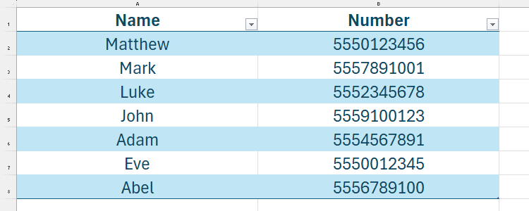
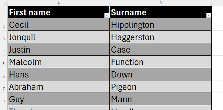
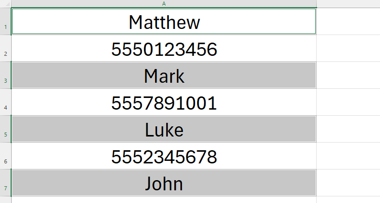
Excel is designed to display data in typical table form.

Lucas Gouveia / How-To Geek |Kamil Zajaczkowski/ Shutterstock
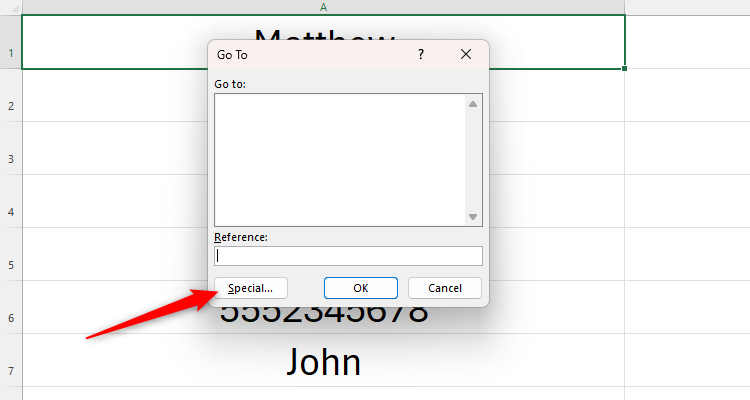
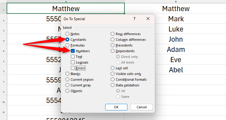
To achieve this, press Ctrl+G to launch the Go To dialog box.
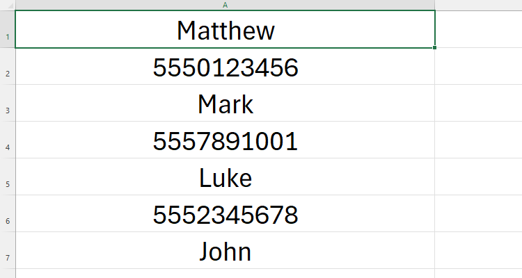
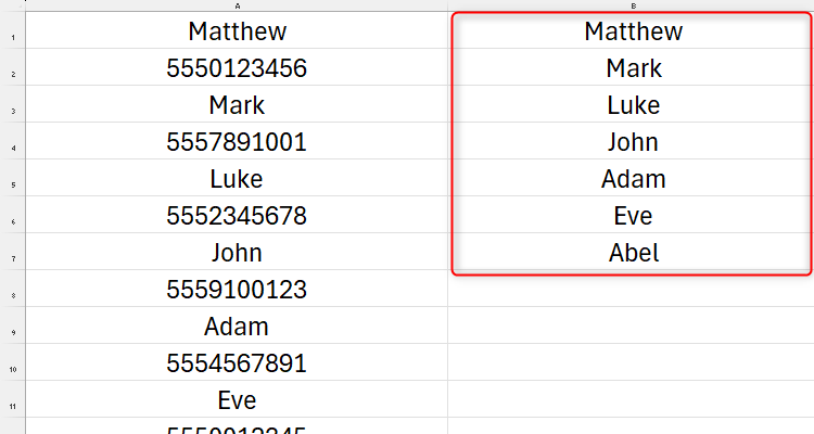
If you have other data in your sheet, first choose the data you want to rearrange.
Then, click “Special.”
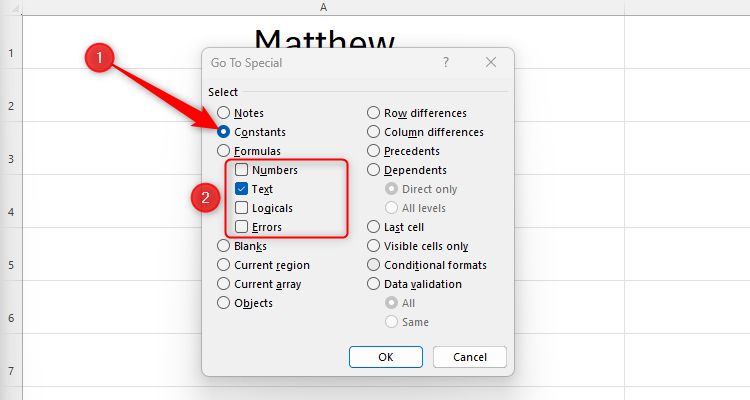
Then, choose the data bang out you want to select.
Then click “OK.”
You will see that only the text is selected.
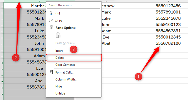
Then, press Ctrl+C to copy the text.
You’ll see that the data has handily pasted without gaps between each cell.
Doing this manually would take a long time and inevitably lead to copying errors.
Luckily, you could do this in just a few steps usingExcel’s transpose pasting function.
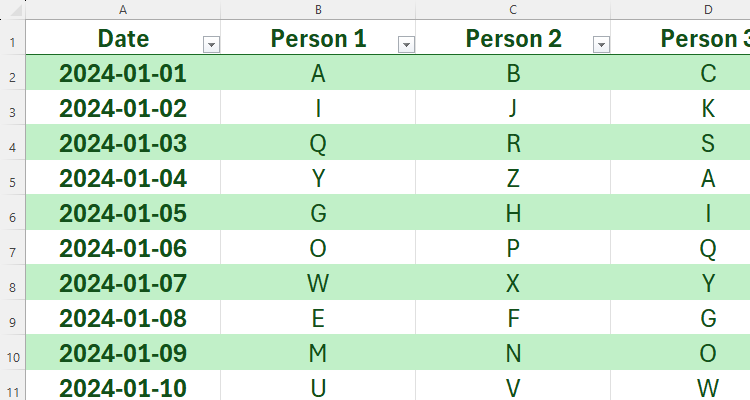
Select all the data in your table (including the header row), and press Ctrl+C.
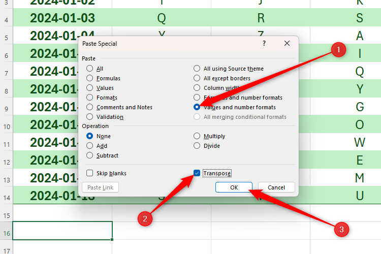
Now, you oughta choose how the data will be converted.
If we don’t pay attention to this, the dates will not transpose accurately.
So, we have clicked the “Values and Number Formats” button.
Finally, click “OK.”
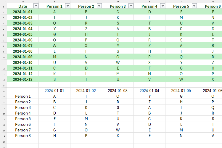
You will then see the data transposed in the position you selected.
you’re able to now delete the original table and format the new one to suit your needs.
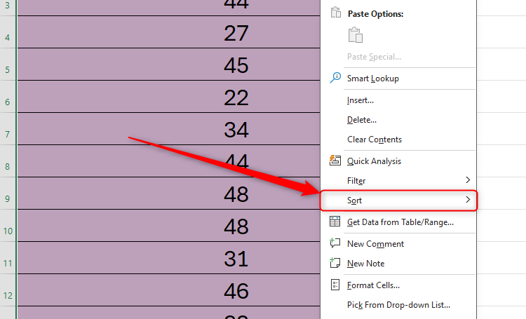
In the menu that appears, hover over “Sort.”
You’ll then see several options.
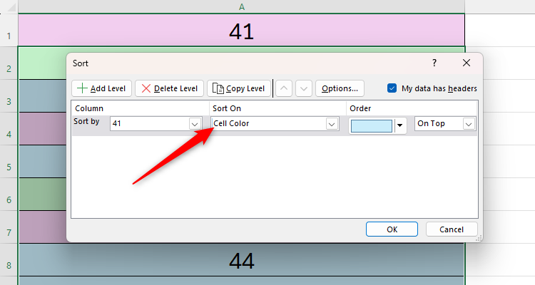
If you do click “Sort,” you will see the following dialog box.
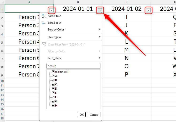
In this case, you gotta add filter buttons to your table.
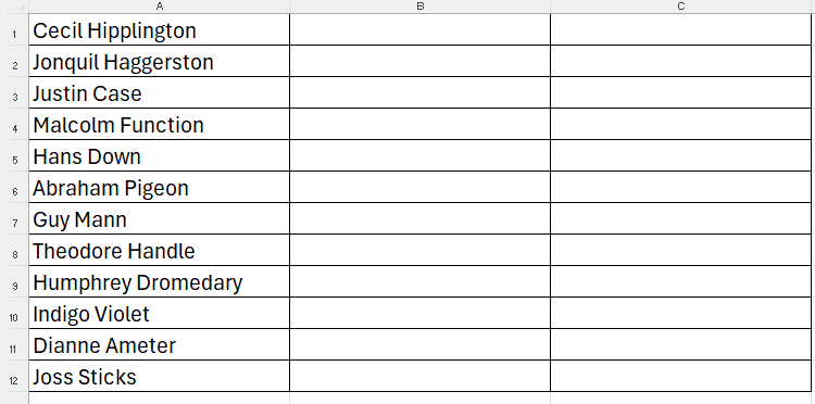
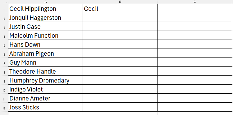
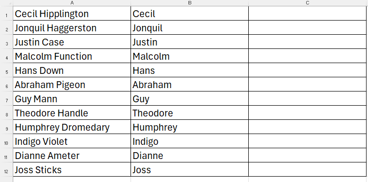
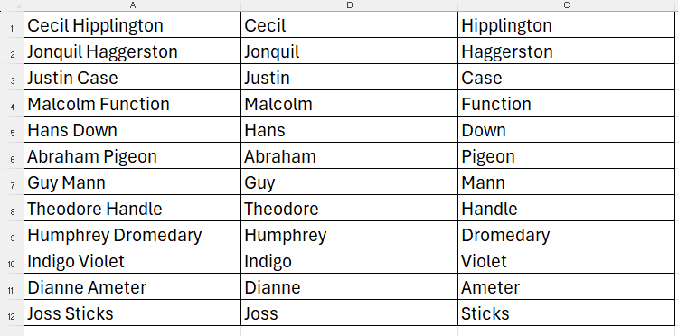
Then, snag the cell directly underneath where you have typed the first entry, andpress Ctrl+E.
It’s no good having nicely arranged data within your spreadsheets if your worksheet tabs are disorganized.
Fortunately, Excel also lets yousort your tabs into alphabetical order.