However, a lot can be said about knowing exactly what it does in different circumstances in Excel.
First, select any cell in your spreadsheet.
In this example, we selected cell D6, and pressed Ctrl+A.
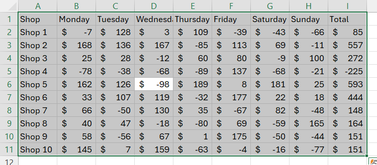
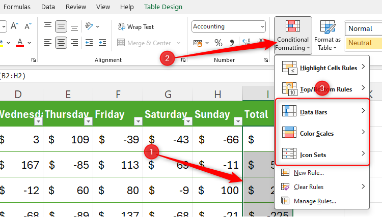
This is useful for formatting only that data range (rather than the whole sheet).
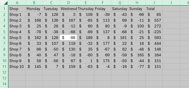
Then, if you press Ctrl+A again, Excel will choose the whole spreadsheet.
This is great for formatting the whole sheet at the same time.
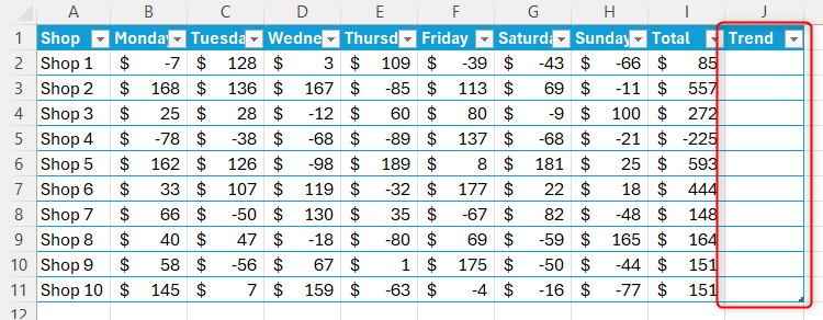
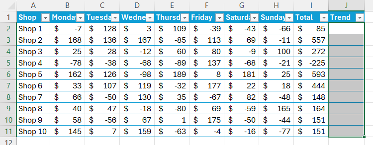
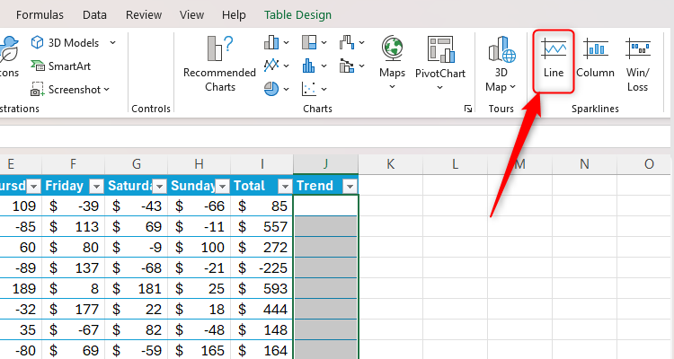
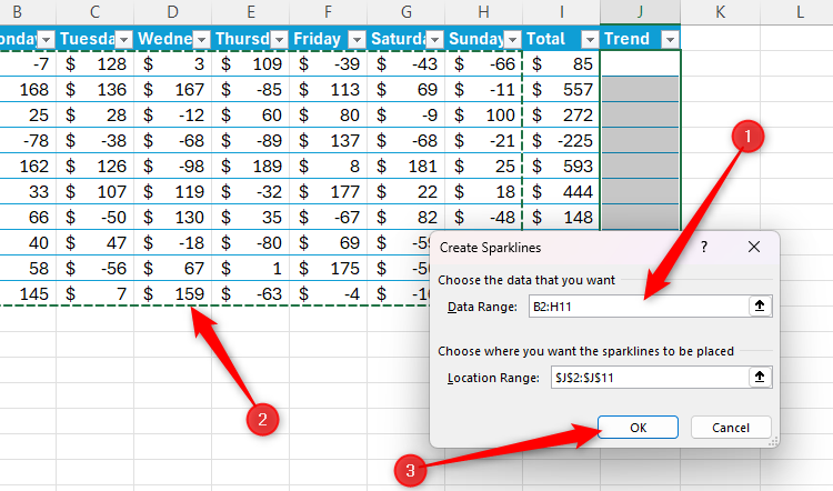
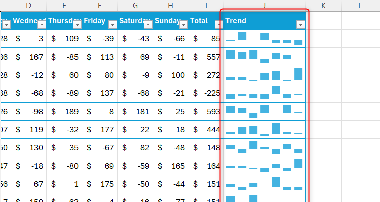
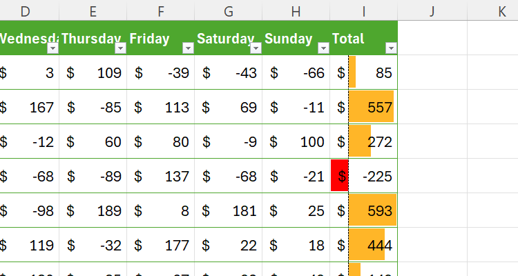
First, pick the cells in column J where you want the trend visualization to appear.
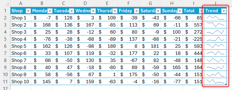
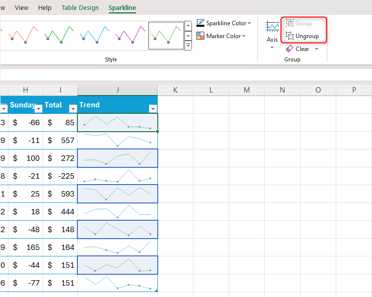
Since they were added together, they will all be formatted in the same way at the same time.
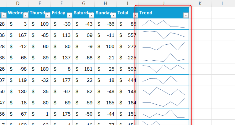
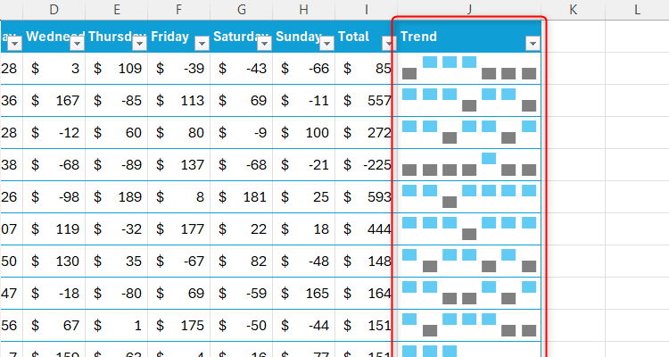
In the example below, we ungrouped every other Sparkline to format them alternately.
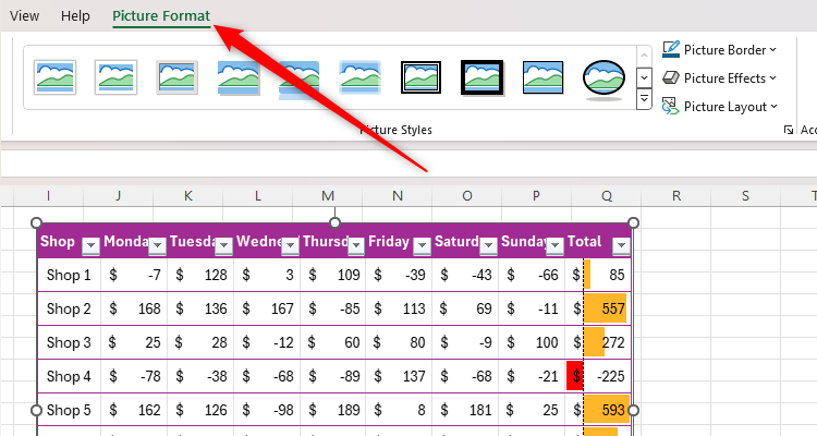
Then, any changes made to the original data will also be reflected in the duplicated data.
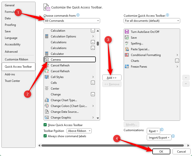
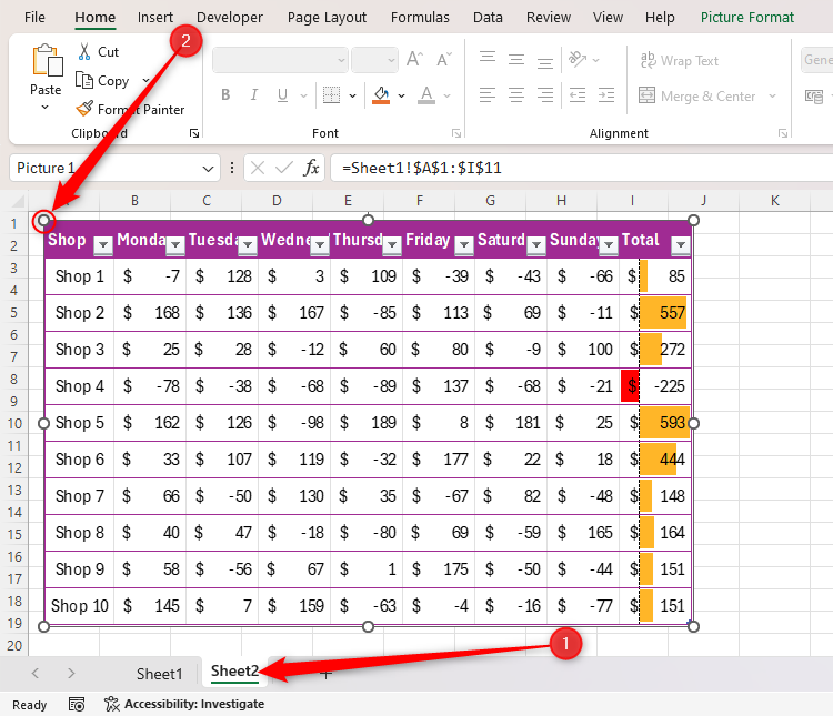
Start by adding the Camera tool to yourQuick Access Toolbar (QAT).
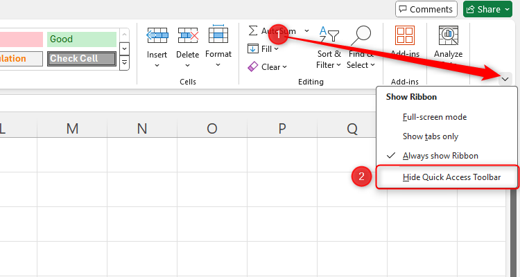
If the Hide Quick Access Toolbar option is available, it means that you already have it showing.
Likewise, if you see the Show Quick Access Toolbar option, click it to activate your QAT.
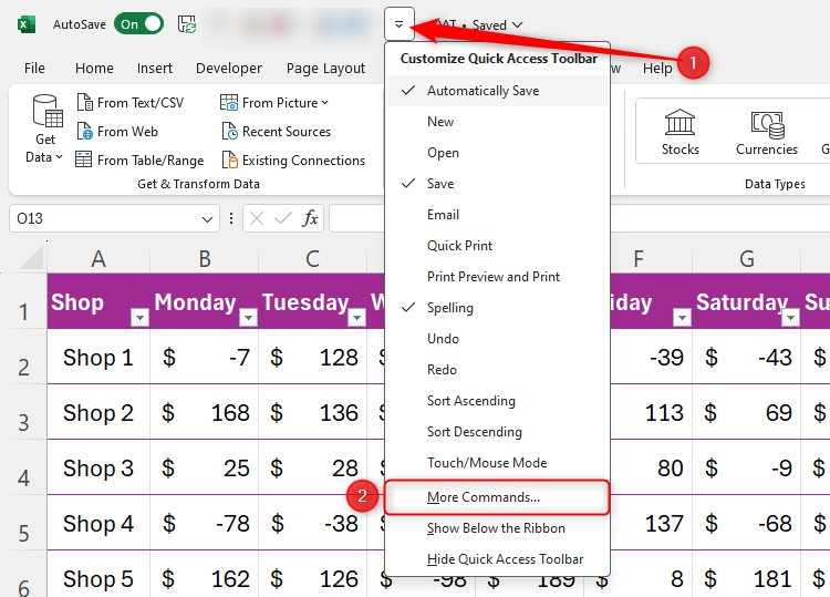
Then, choose the QAT down arrow and click “More Commands.”
Then, click “OK.”
You will now see the Camera icon in your QAT.
This will copy the selected cells and everything in front of them as an image.