Where the methods are slightly different, I’ve added a note to explain this.

The Issue

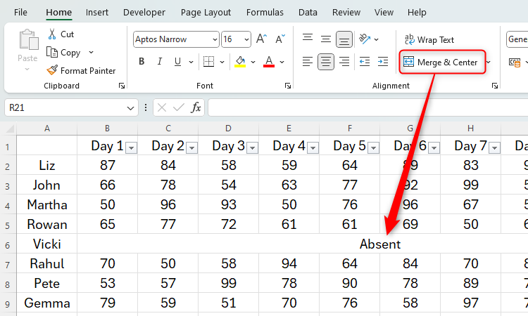
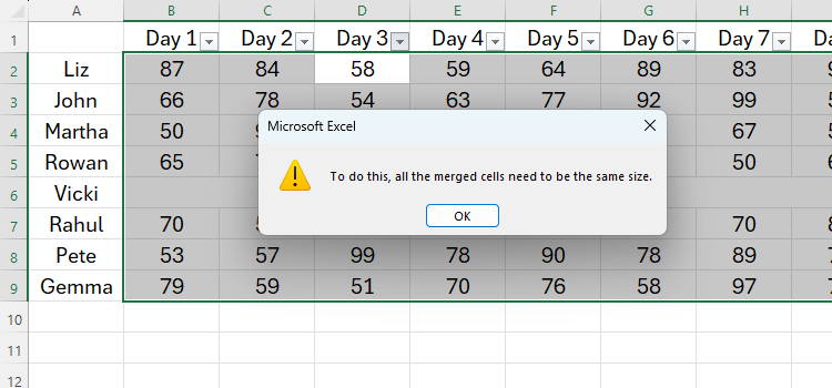
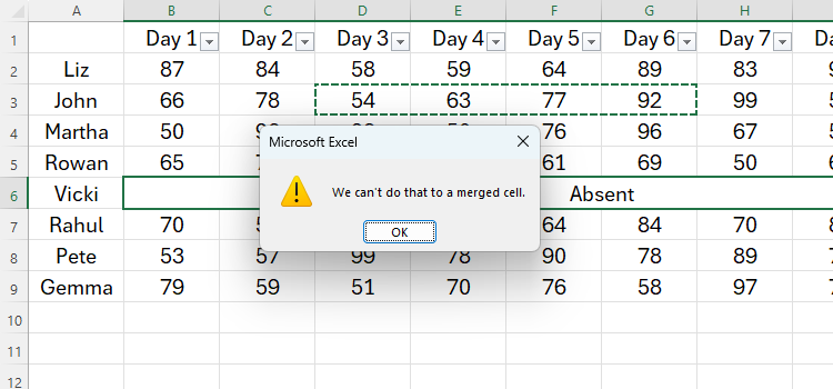
However, merging cells causes issues when you attempt to perform actions with your data.

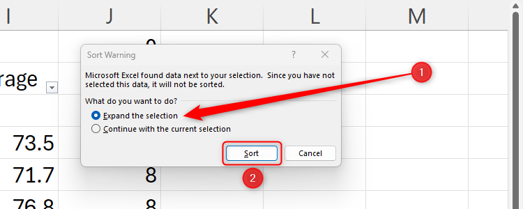
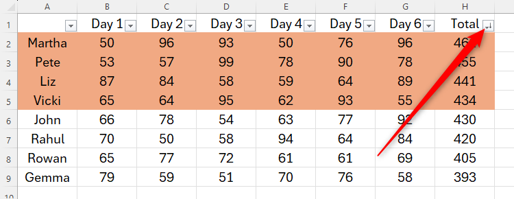
First, if you attempt to sort your data, you’ll receive an warning pop-up.

Data in Excel with one row merged and centered.

The Solution

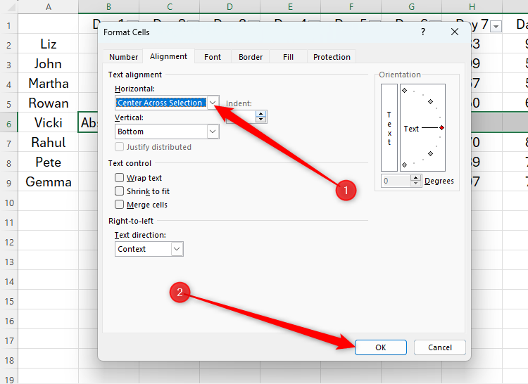
First, click “Merge and Center” to unmerge the cells.

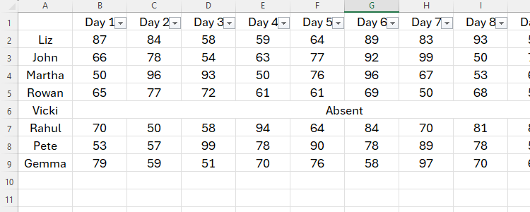
“Center Across Selection” only works across rows, and not down columns.

There’s a really easy way to deal with these issues.

An Excel spreadsheet with an error message reading ‘To do this, all the merged cells need to be the same size.'

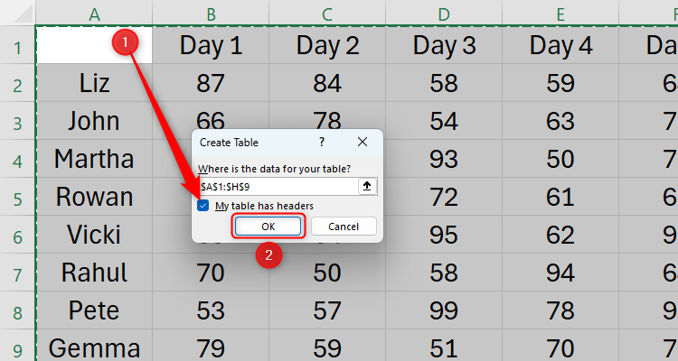
First, select all the data in your original, unformatted table, including your header columns and rows.

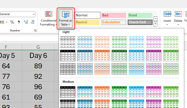
To do the same in Excel for the web, select your data and click Insert > Table.

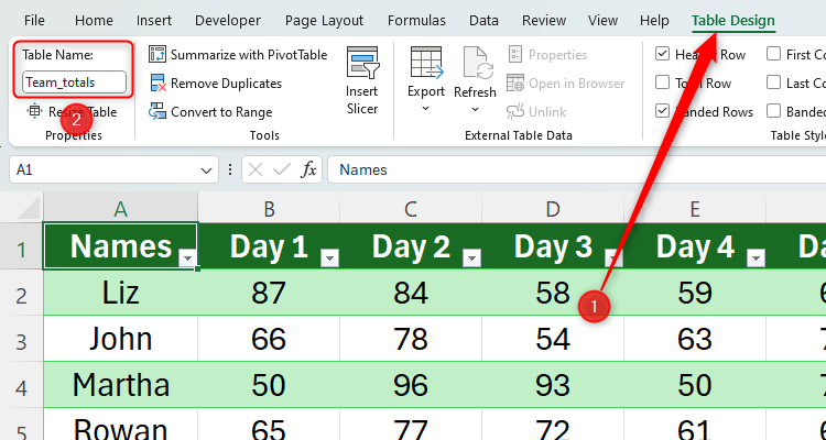
Finally, Excel would automatically apply formulas to any new rows I add.

An Excel spreadsheet with an error message reading ‘You can’t do that to a merged cell.'

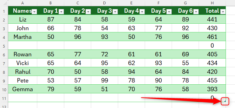
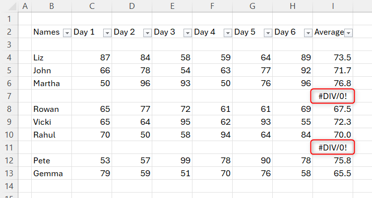
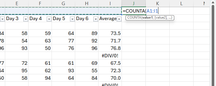
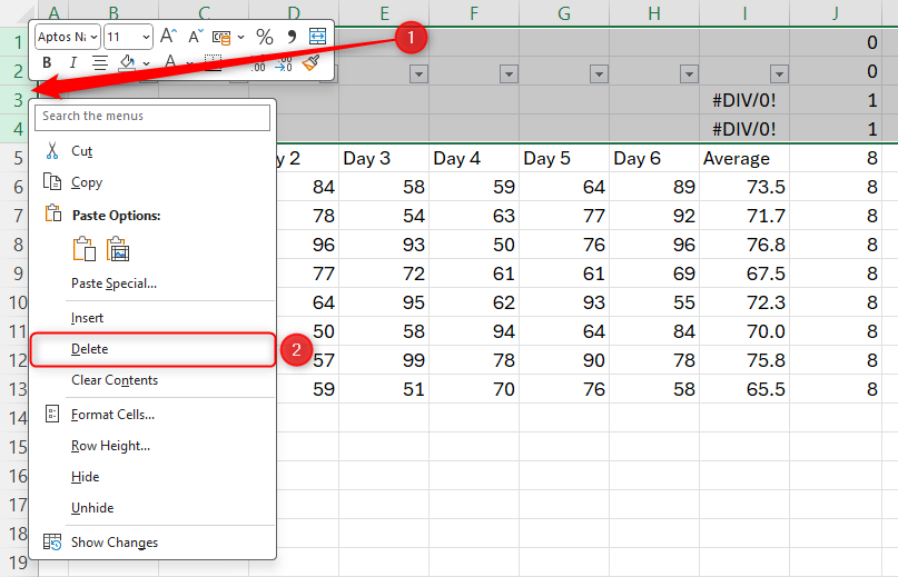
However, if you have lots of blank rows, you could use the COUNTA function to rectify this.

Then, press Enter.

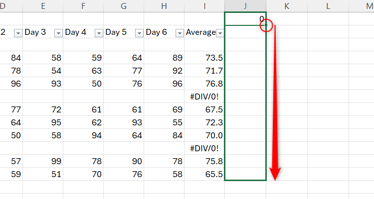
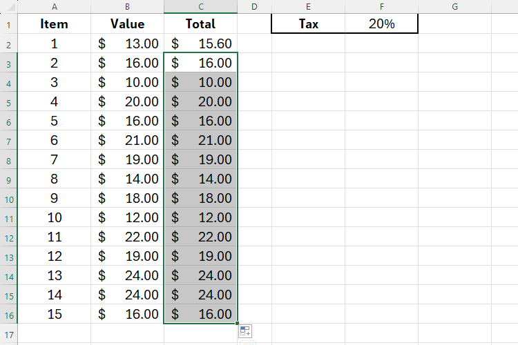
Next, drag the AutoFill handle to the bottom of your data.

The Excel Format Cells dialog box with the Alignment tab opened. The Horizonal option is changed to ‘Center Across Selection,’ and the OK button is highlighted.

In the Sort Warning dialog box, choose “Expand The Selection” and click “Sort.”

Finally, delete your COUNTA column.

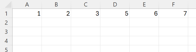
Excel’s AutoFill can recognize patterns in your data and fill in the rest for you.

An unformatted Excel table with one of the rows containing the word ‘Absent’ in the center of the row.

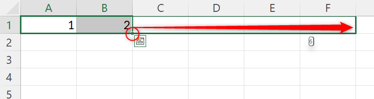
Start by typing the first two values in your data.

Then, select these values and use the AutoFill handle to complete the data.

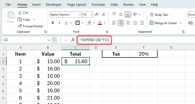
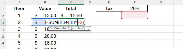
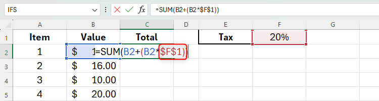
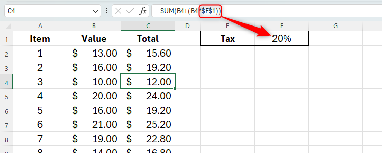
In this example, I have referenced cells B2 and F1 when calculating the total value in cell C2.

An Excel table with alternate rows manually colored. An additional row has been added to the center of the table, so the rows are no longer alternately colored.

Relative referencesassess the relative positions between cells.

Then, when I AutoFill the remaining totals, Excel will continue to reference F1 to make the calculation.

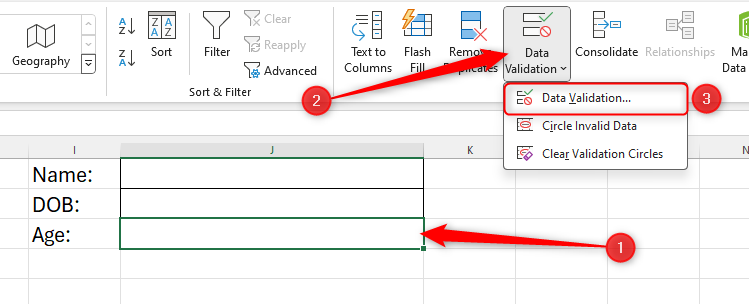
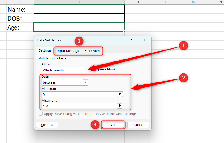
Excel lets you control what other people can enter into a spreadsheet throughdata validationandlocked cells.

An Excel table with its manual formatting altered due to column H having been sorted.

Data validation dictates what throw in of data can be input into a cell.

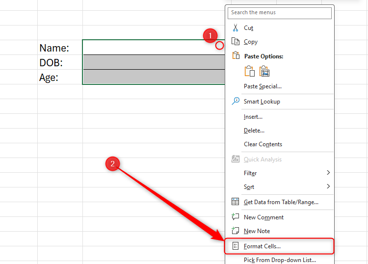
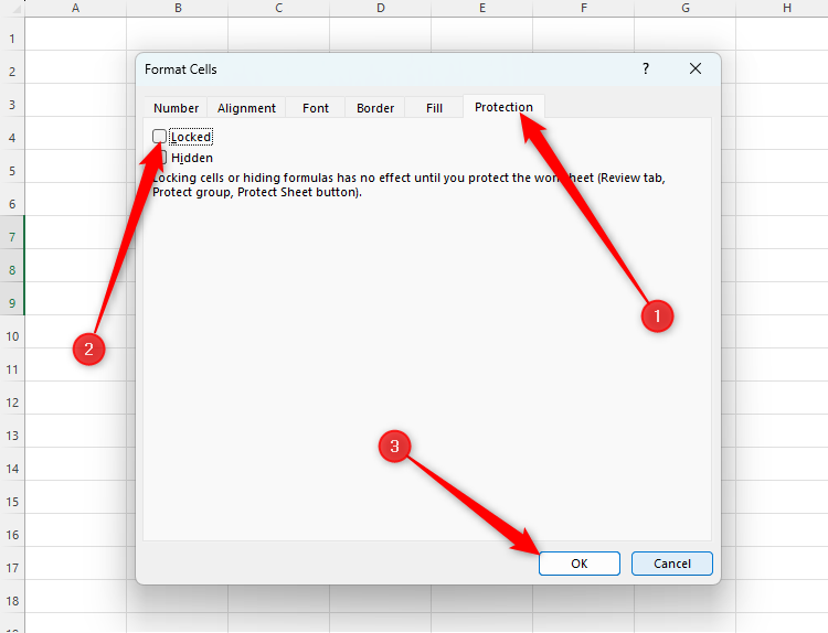
To do this, select and right-click those cells, and click “Format Cells.”

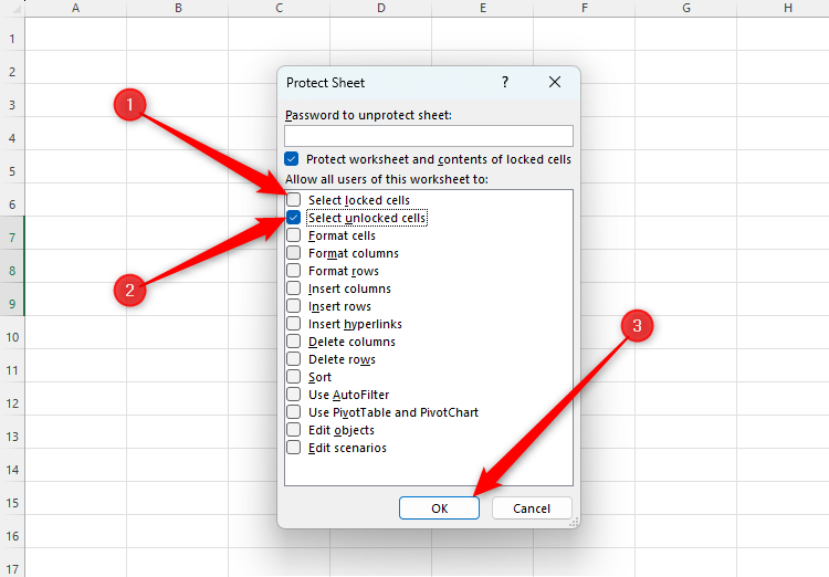
you might also enter a password if you wish.

An Excel worksheet with data selected and the Format As Table option highlighted.

To reverse this action, click “Unprotect Sheet.”

As with any software, especially the Microsoft 365 suite of programs, practice makes perfect.

Excel’s Create Table dialog box with the My Table Has Headers checkbox checked and the OK button highlighted.

An Excel table with the Table Name changed to Team_totals in the Table Design tab on the ribbon.

A formatted table in Excel with new rows added in the center and at the bottom of the table. The table expansion handle in the bottom-right corner is indicated with an arrow.

An Excel spreadsheet with row 1 and column A left blank. There are also some other rows containing no data.

An unformatted table in Excel containing blank rows, which cause the DIV0 error message to appear when performing an AutoFill operation.

A circle shows where to right-click to bring up a row’s options in Excel, and the ‘Delete’ option is selected.

An Excel sheet with the COUNTA formula typed into the highest cell to the right of the data.

An Excel spreadsheet with the AutoFill handle highlighted and an arrow indicating the downwards direction of the AutoFill.

An Excel sheet with column J selected, and the ‘Sort Smallest To Largest’ option in the Sort and Filter menu highlighted.

An Excel sheet showing the Sort Warning dialog box, and the ‘Expand The Selection’ radio box is checked.

An Excel sheet with the top four rows selected for deletion.

An Excel sheet with numbers typed across row 1. The number 4 has been accidentally omitted.

An Excel sheet with the numbers 1 and 2 typed into cells A1 and B1 respectively, and the AutoFill handle is highlighted with an arrow pointing in the direction to click and drag the AutoFill handle.

An Excel sheet with a formula in C2 which references cells B2 and F1, as seen in the formula bar at the top.

An Excel sheet showing calculations that have not worked.

An incorrect cell reference in Excel.

An Excel formula containing $F$1 as an absolute reference.

An Excel worksheet with a formula in the formula bar containing an absolute reference to cell F1.

A cell in Excel is selected and the Data Validation option is highlighted.

Excel’s Data Validation dialog box with the different options highlighted.

An Excel sheet with three cells selected and right-clicked, and the Format Cells option highlighted.

The Format Cells dialog box in Excel with the Protection tab open, ‘Locked’ unchecked, and the OK button highlighted.

Excel’s Protect Sheet dialog box with Select Locked Cells unchecked, Select Unlocked Cells checked, and the OK button highlighted.