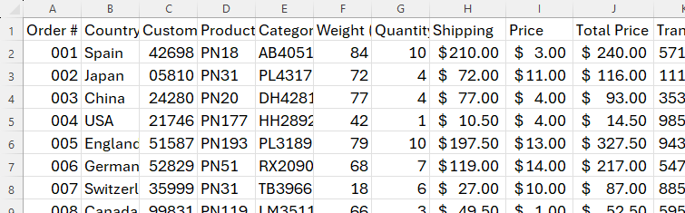
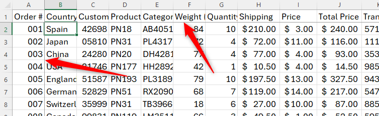
This unformatted spreadsheet has several readability issues which we’ll address throughout this article.
An example will make this clearer.
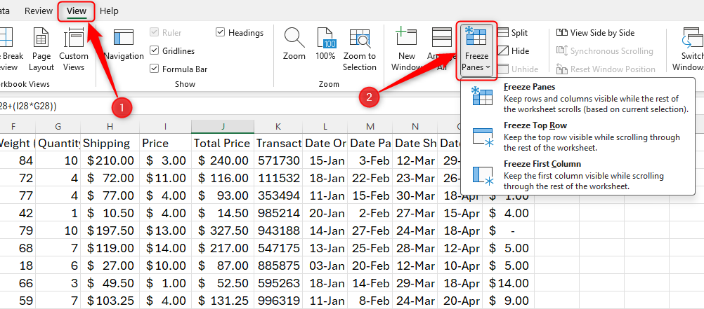
Excel will then draw a thicker line to demonstrate where the freezing has taken effect.

Lucas Gouveia / How-To Geek
Now, when you scroll down or across, you’ll see that the headers remain viewable.
Pressing Ctrl+Z (undo) will not work.
After all, Excel already has its in-built gridlines to help you differentiate between cells.
Instead, color your cells or use horizontal borders only.
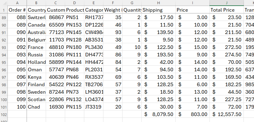
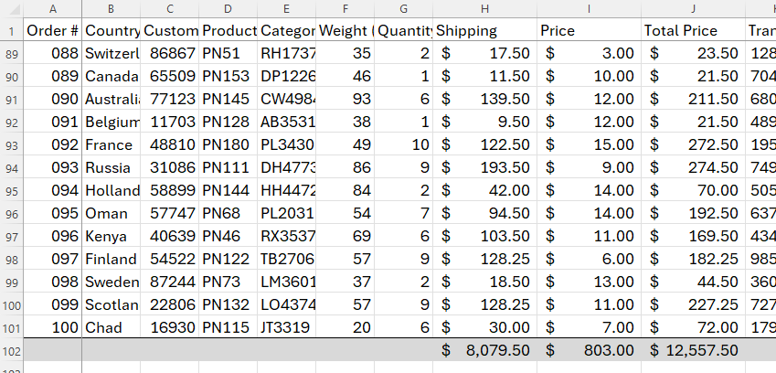
First, opt for row you want to affect (in our case, row 102).
For more border or color options, right-choose the row number, and click “Format Cells.”
Whichever color you choose, use variants of that same color throughout your spreadsheet (tip 3).
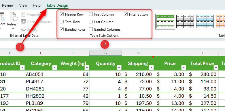
Furthermore, you might let Excel create the table formatting for you (tip 5).
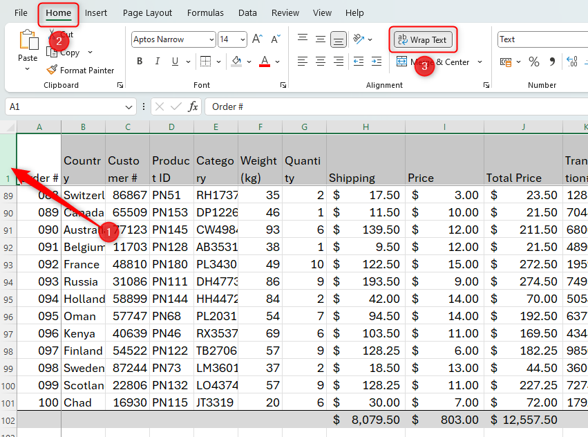
This means that the text runs onto the next line to fit into the chosen cell width.
To do this, highlight the header row, and bring up the “Home” tab.
Then, in the Alignment group, click “Wrap Text.”
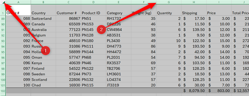
So, the second step is toadjust the column widths.
To do this, highlight all cells in the worksheet by clicking the top-left cell reference square.
Glance at your table to see to it you’re happy that the text and data fit nicely.
If you’re not, simply adjust them again until they look great.
Once you’ve achieved a suitable cell width, click anywhere on your sheet to deselect the cells.
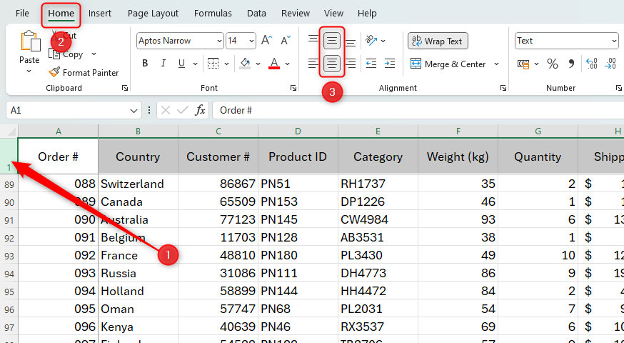
We’d also recommend that you center-align your headers vertically and horizontally to add that extra professional quality.
opt for header row and click both center alignment icons in the Alignment group on the Home tab.
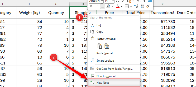
In Excel, by default, text aligns to the left and numbers align to the right.
To get around this, right-poke the relevant cell and click “New Note.”
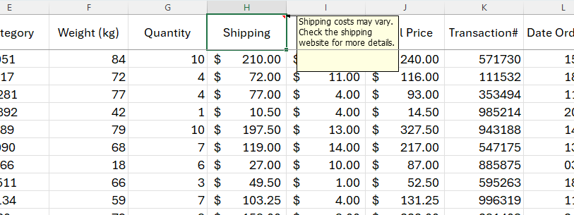
Hover over any cells containing this red marker to see the note.
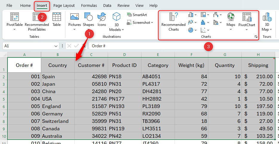
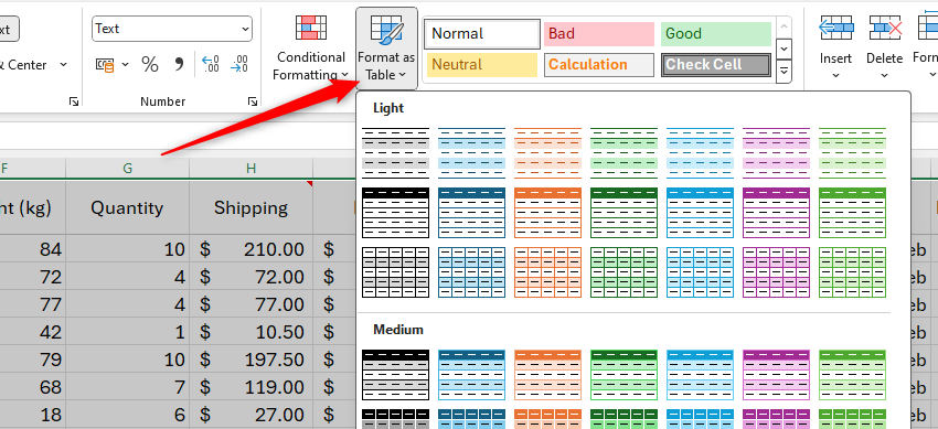
you’re free to also tell Excel toformat your tables.
To do this, highlight all the data in your table, including the header row or column.
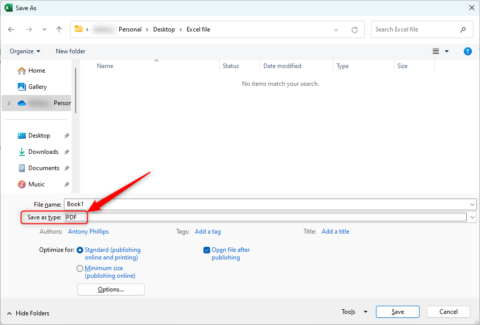
To keep your layout intact,back up your worksheet as a PDF.