Do you find yourself endlessly scrolling or jumping from one tab to the other?
Stop there, because this hack will patch this up for you.
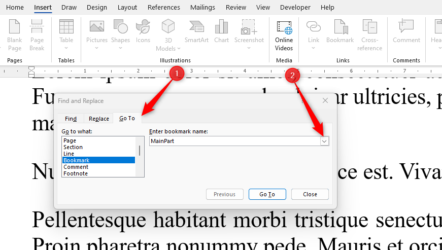
What is a Bookmark (in Word)?
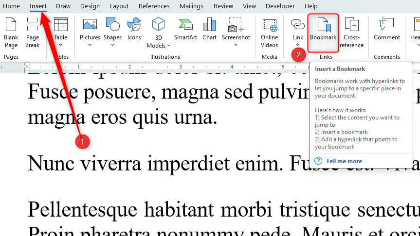
Here, it’s possible for you to give your bookmark a name (with no spaces).
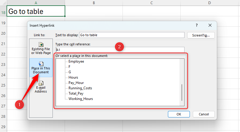
It’s also great for creating hyperlinks to certain parts of your work.
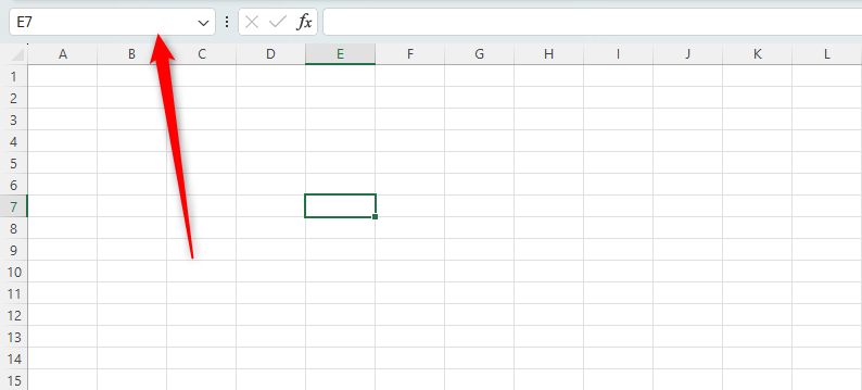
For example,
would take us to Sheet 2, cell G5.
it’s possible for you to also use the name box to highlight a range of cells.
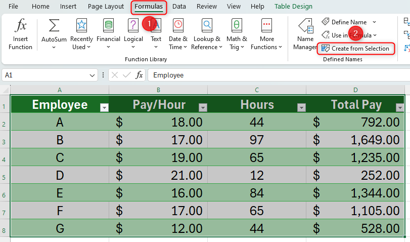
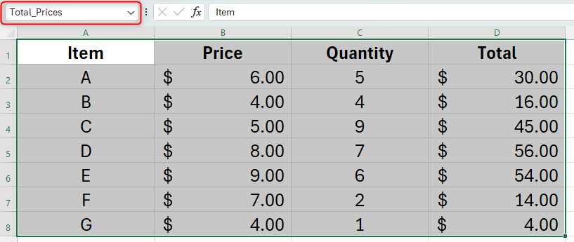
What’s more, you’re able to also name a range of data.
Let’s say you have an important data range in your large workbook that you should probably view often.
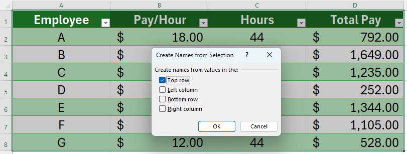
Simply opt for data and give it a name.
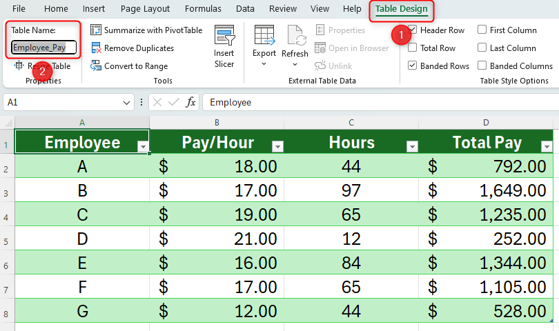
You’ll need to use a slightly different method to name a formatted table.
Go to the bottom of this section for instructions on how to do this.
Excel doesn’t like spaces in names.
you’re able to also name other elements in your workbooksuch as charts or illustrationsin the same way.
If you prefer to use keyboard shortcuts, press F5 to bring up the Go To dialog box.
you could also create a hyperlink to named cells in your workbook.
We will discuss this more in the final section of this article.
Select any cell within your table, and hit the “Table Design” tab on the ribbon.
Head to the Properties group and change the name of your table, before pressing Enter.
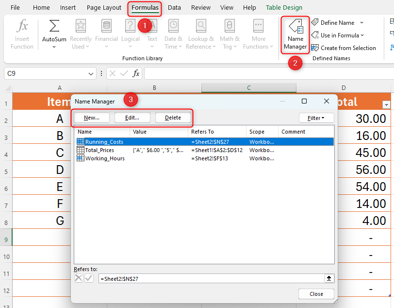
Or, maybe, you’re gonna wanna change a name you’ve already assigned.
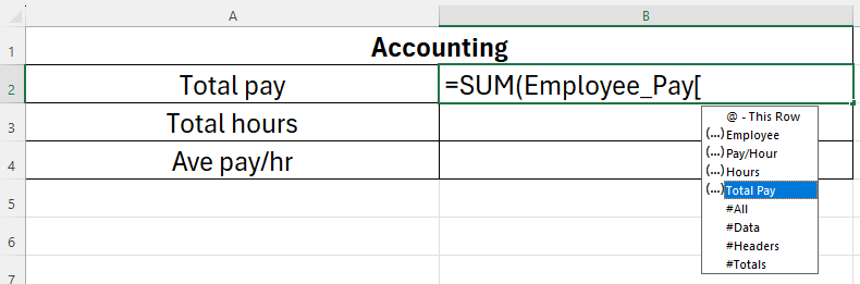
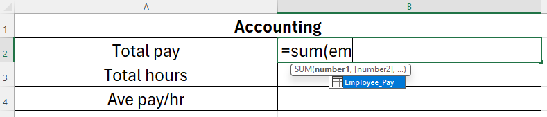
Start by typing the calculation you want to create.
In our case, we want to sum the employees' pay.
Now, begin typing the name of the data range.
In our case, it’s Employee_Pay.
You’ll notice that the name you have given the data range appears.
Double-smack the data name.
This time, Excel will bring up each column name within your named table.
Double-hit the column name, terminate the square parenthesis, and terminate the formula parenthesis, before pressing Enter.
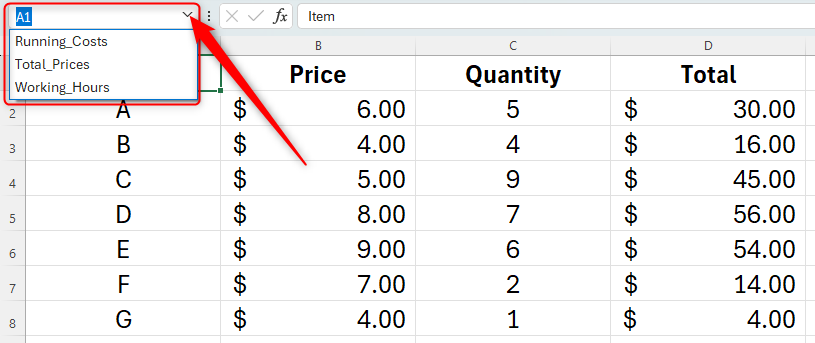
If you have a particularly large spreadsheet, you may not remember which names refer to which ranges.