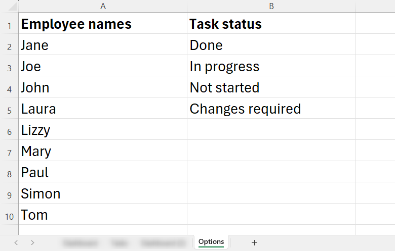
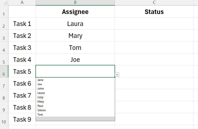
First, create the options to appear when you click a drop-down cell.
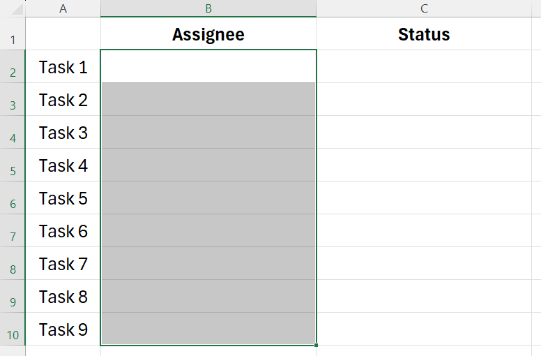
Now, create another sheet where the tasks will be managed and rename itTasks.
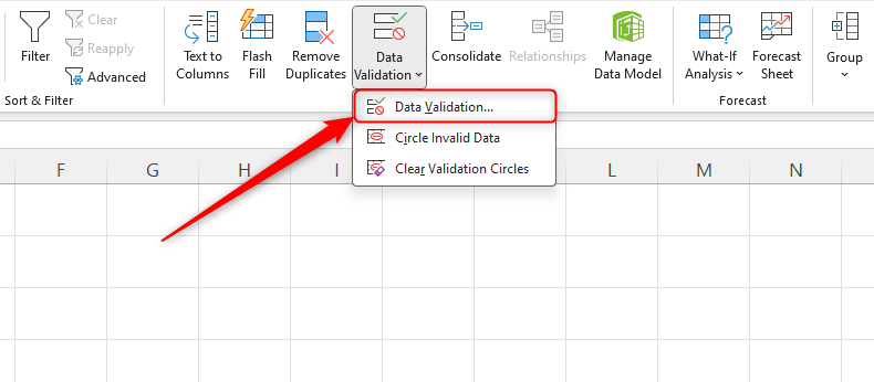
Next, in the Data tab on the ribbon, click “Data Validation.”

Lucas Gouveia / How-To Geek |Kaspars Grinvalds/ Shutterstock
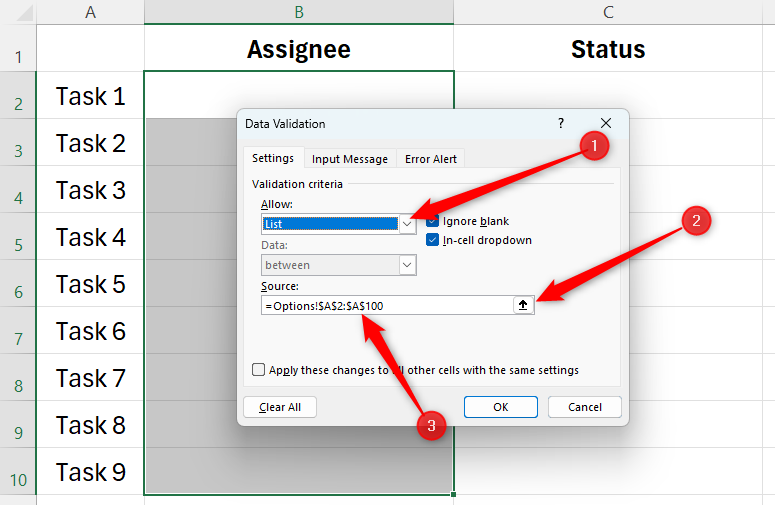
In the Allow field of the Data Validation dialog box, choose “List.”
Excel has tools for creating simple Gantt charts, but they are less adaptable than those created from scratch.
Keep reading to see how to create a more dynamic Gantt chart.
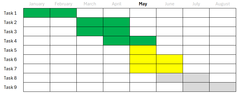
On this new sheet punch in the tasks' names on the left and the months at the top.
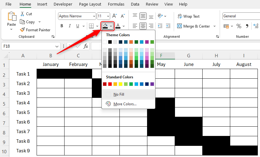
Next, map out your proposed timings using manual color fill.
opt for first cell you want to color, hold Ctrl, and then opt for remaining cells.
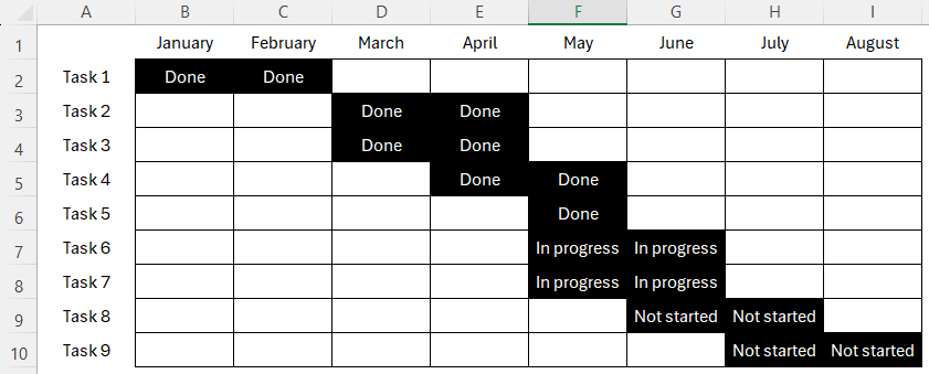
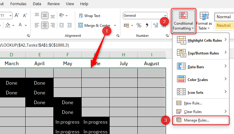
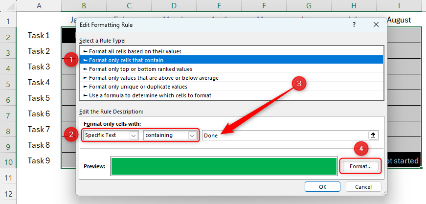
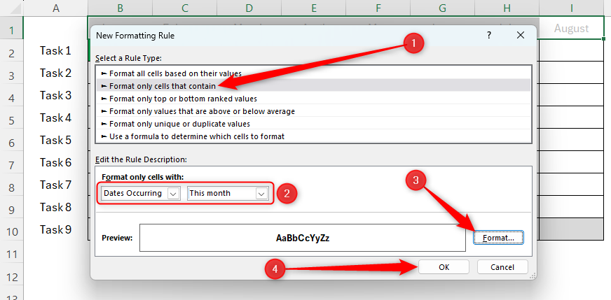
Finally, use Conditional Formatting to color the cells based on the values they contain.
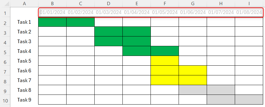
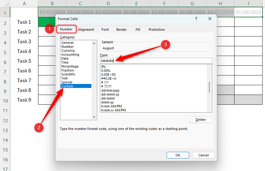
So, for example, replace the text in the cell containing January with01/01/2024.
Then, do the same for February, beforeusing AutoFill to complete the remaining months.
Doing this tells Excel that these are dates, and not just text.
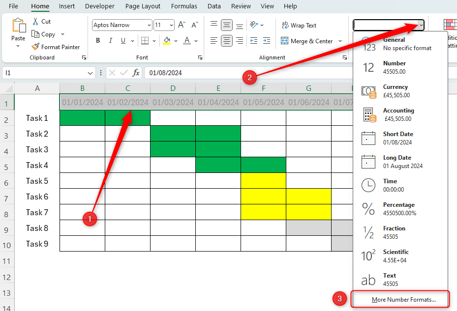
Next, change the font color of these dates to gray.
Then, in the pop in field, typeMMMM.
Then, click “OK” to see the result.
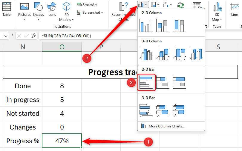
Remember to change the number format of this cell to a percentage.
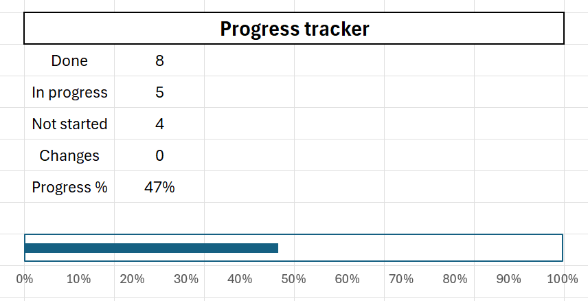
Remove the gridlinesto make your progress bar easier to read and look more professional.
First, bang out the start and due date manually using a date format that suits your region.
Excel will automatically convert this to a date format, and you canamend the date formatif required.
Next, add today’s date by typing
and pressing enter.
Then, calculate the weeks elapsed by dividing the days elapsed by seven.
Again, calculate the weeks remaining by dividing the days remaining by seven.
Finally, create a 2-D bar chart using the method described in the previous section.
Now you’ve created the perfect spreadsheet for project management, considerusing Excel to help you monitor your budgets!
![]()
![]()
![]()
![]()
