Here’s everything you better know about how to do it.

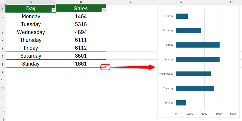
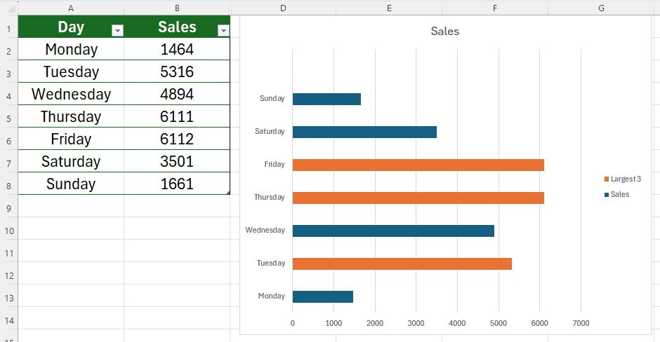
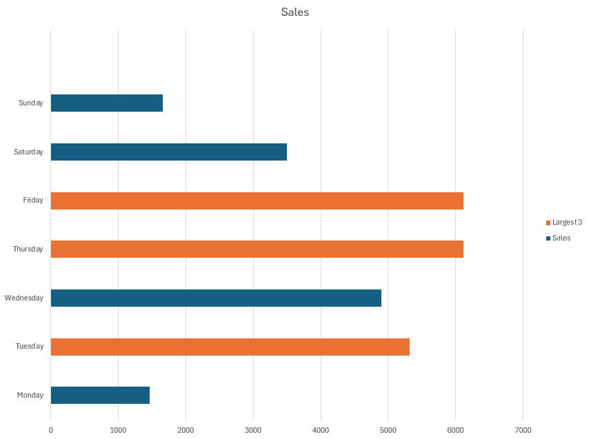
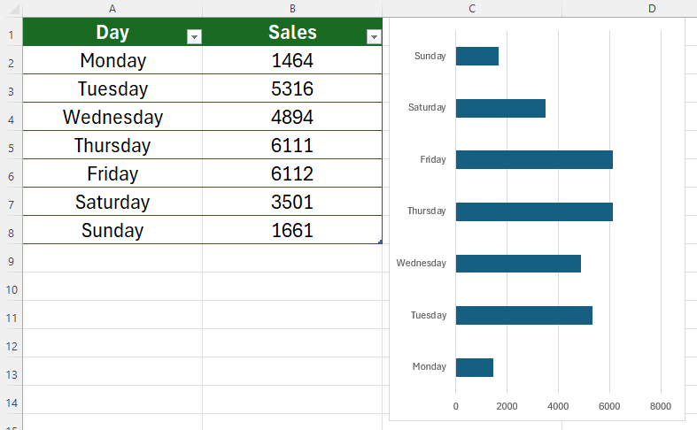
Here’s what our chart will look like after running through the steps in this article.

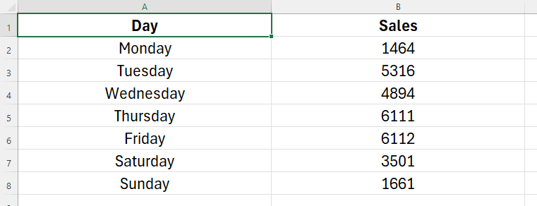
Step 1: Prepare Your Data

Start by creating your Excel table.

A tablet with an Excel spreadsheet and a chart highlighting the maximum and minimum values.

Lucas Gouveia / How-To Geek |Kaspars Grinvalds/ Shutterstock

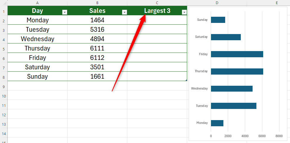
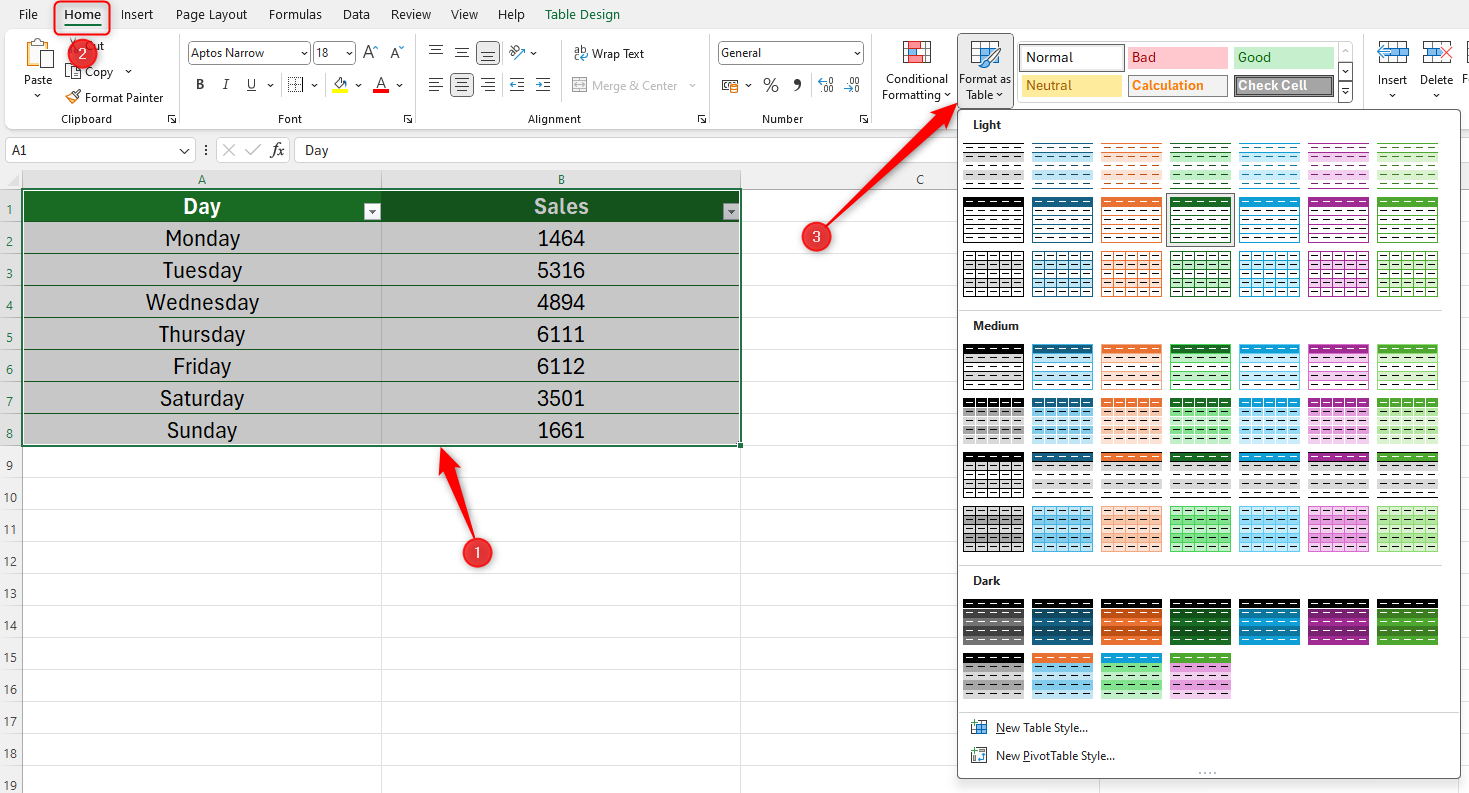
Then, choose a design that works for you.

As you’re able to see, we’ve chosen a simple green design.

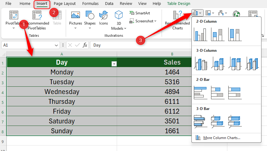
Step 2: Create Your Chart

Now, you could create the chart for your table.

A completed sales chart with the three highest-value bars colored orange, and the remaining data bars colored blue.

Select all the data in your table (including the header row).

For our data, we’ve chosen a 2D clustered bar chart.

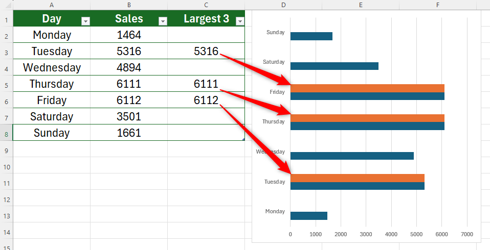
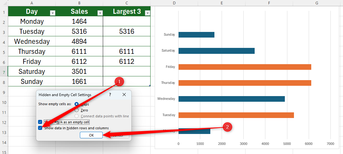
In our example, we want to highlight the three largest values.

An unformatted Excel table with the day of the week in column A and number of sales in column B.

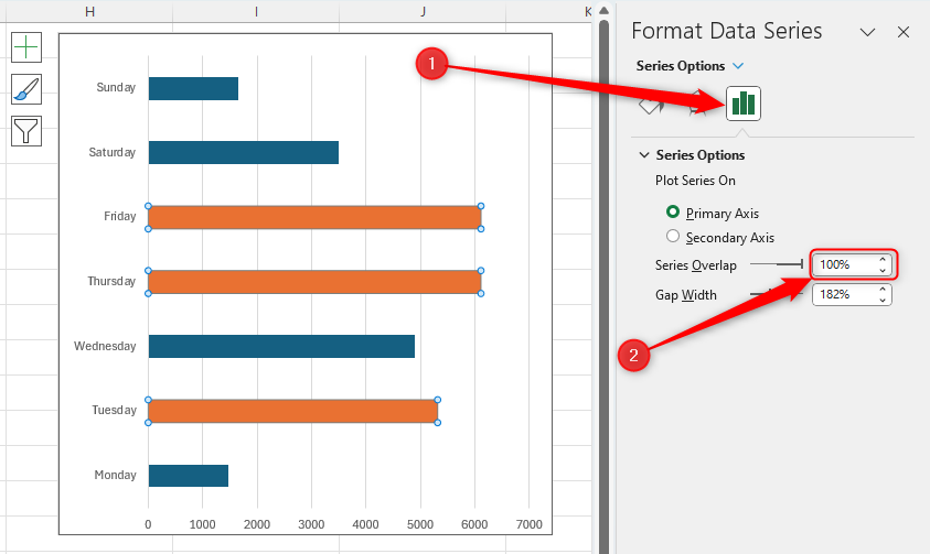
Now, specify how many values you want to extract.

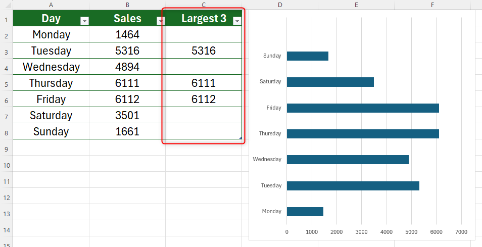
After you have typed your formula, press Enter.

If the cell remains blank, it means that it’s not one of the three highest values.

An Excel table with the Format As Table drop-down opened.

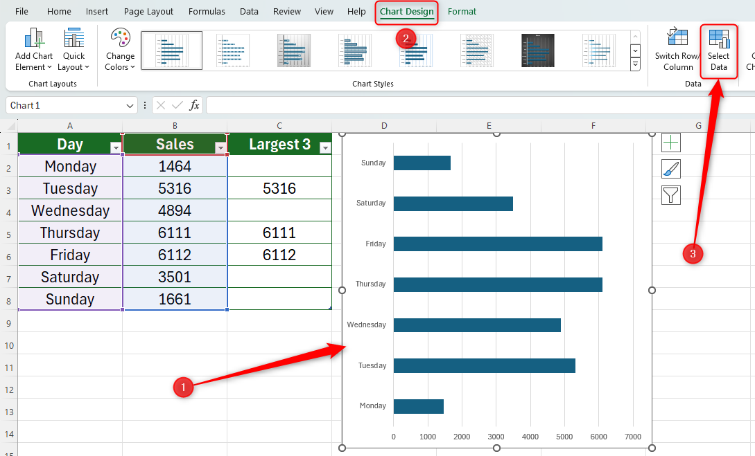
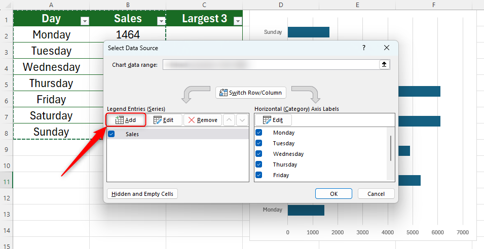
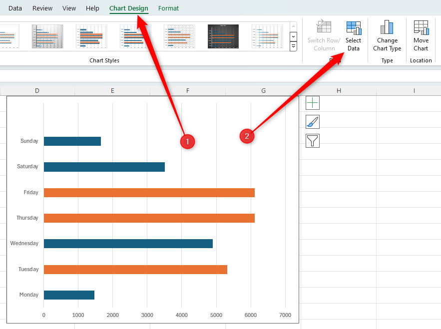
snag the chart, open “Chart Design” on the ribbon, and click “Select Data.”

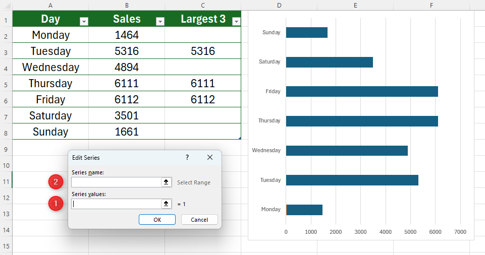
In the Edit Series window, you will see two fields to complete.

First, clear both fields of any information they already contain.

An Excel worksheet with data in a table selected, and the chart drop-down selector opened.

In our case, we would highlight cells C2 to C8.

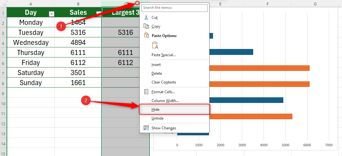
Then, hit the Series Name field box and go for the table header for the new data range.

In our case, we would select cell C1 (Largest 3).

An Excel worksheet with a table on the left and a corresponding chart on the right.

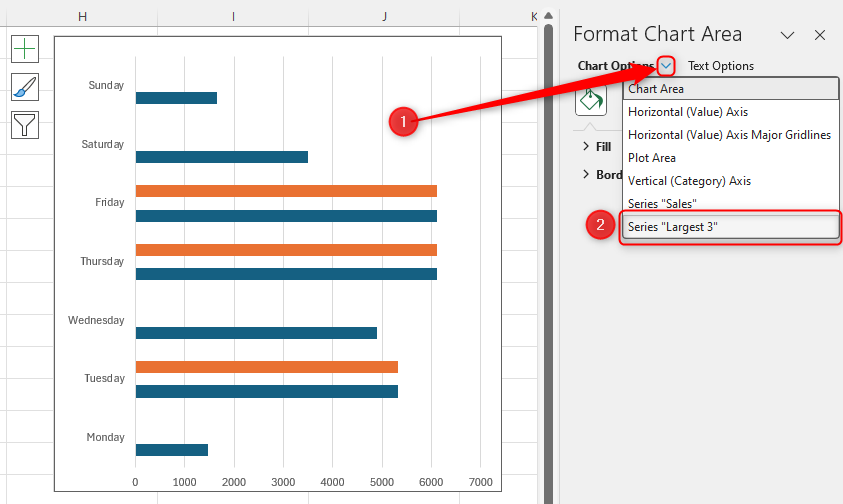
You will now see the final outcomeyour chart highlights the max three values in your Excel chart!

First, you should probably check that your chart includes data that is contained within hidden cells.

Here’s our finished product!

An Excel table with the table handle highlighted and an arrow showing the direction to click and drag the handle.

An Excel table with three columns and an arrow pointing to the header name (Largest 3) in the third column.

An Excel sheet containing a table with the largest three values extracted into an additional column.

An Excel sheet with a chart selected and ‘Select Data’ highlighted.

An Excel sheet with the Select Data Source dialog box open, and ‘Add’ highlighted.

The Edit Series dialog box in Excel with Series Values labelled as ‘1’ and Series Name labelled as ‘2’.

An Excel chart next to a table. There are three arrows, each pointing from the new series of data in the table to its corresponding bar in the chart.

An Excel chart with the Format Chart Area pane open and a drop-down arrow highlighted. The series name is also highlighted.

An Excel chart with the Series Options highlighted and opened, and the Series Overlap set to 100%.

An Excel spreadsheet with a chart selected, and ‘Select Data’ being clicked.

‘Show Data In Hidden Rows And Columns’ in the Hidden And Empty Cells Settings dialog box is checked.

Column C selected with a right-click, and ‘Hide" highlighted in the drop-down options.

An Excel sheet with a chart whose top three values are a different color, and a table with the extra column hidden