Quick Links
An easy way to make numbers stand out in Google Sheets is withconditional formatting.
So as your values change, you could see those numbers pop without any extra work.
We’ve shown you how to useconditional formatting based on dateand how touse it for certain text.
So let’s get back to the most basic usage of the feature and automatically highlight values with it.
Any rules you set up apply only to the current spreadsheet.
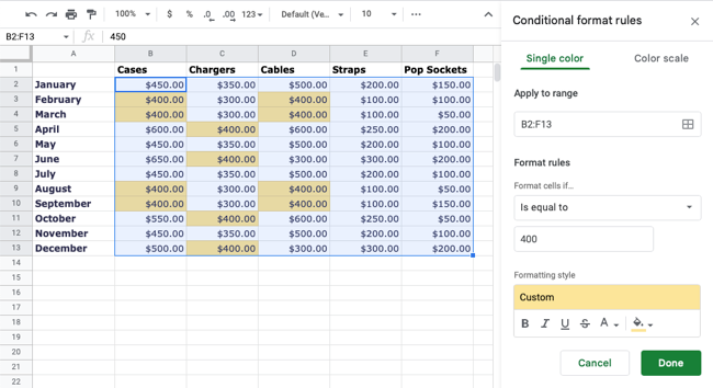
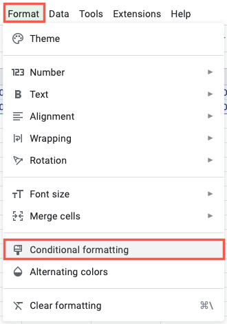
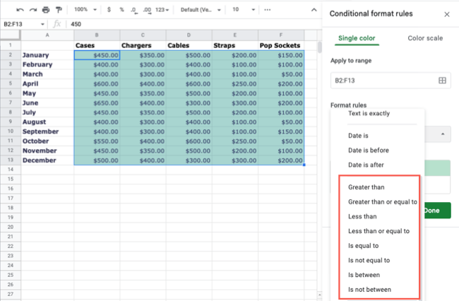
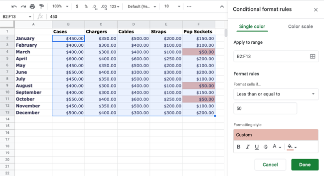
Go to the Format tab and choose “Conditional Formatting.”
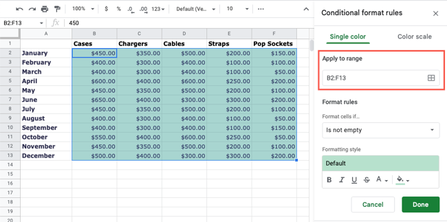
This opens a sidebar on the right for you to set up a rule.
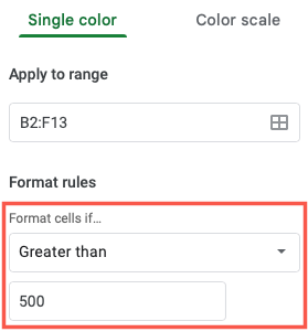
snag the Single Color tab at the top and confirm the cells in the Apply to Range box.
Next, pick the criteria you want to use in the Format Cells If drop-down box.
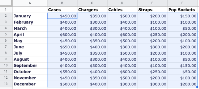
As an example, we’ll choose Greater Than to highlight sales higher than $500.
After you pick the criteria, you’ll add the corresponding value(s) in the box beneath.
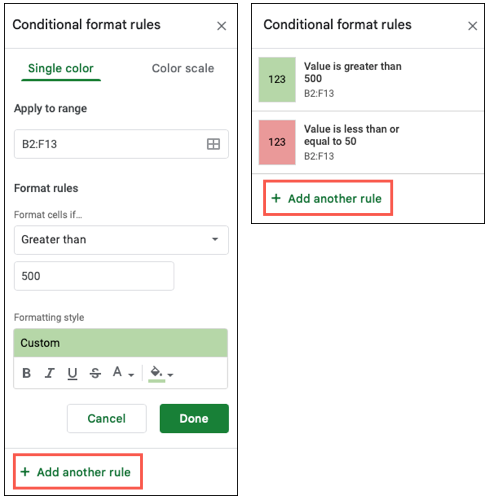
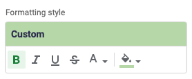
you’re able to also use a combination of styles if you like.
So, you’re able to pick both a bold font and a green cell color.
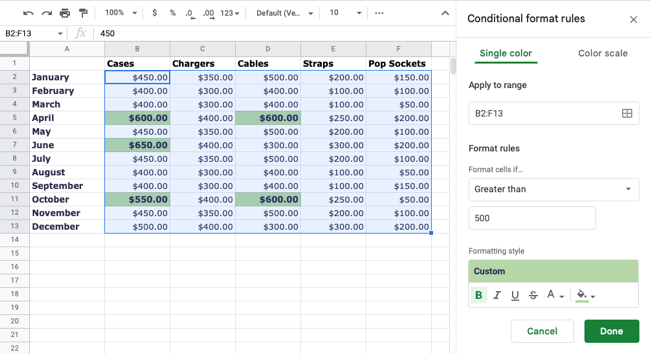
As youselect the formatting, you’ll see your sheet update for a nice preview of your selection.
This lets you make adjustments before you save the rule.
When you’re happy with the highlighting, click “Done” to apply the rule.
You should see the cells that meet your criteria highlighted.
And, if you make any changes to those cells that affect the criteria, they automatically update.
Conditional Formatting Examples
Let’s look at more exampleuses for conditional formattingbased on values.
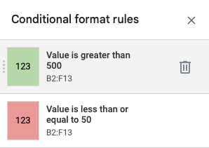
Here, we can see our lowest sales, those equal to or less than 50.
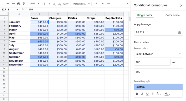
Maybe you want to see specific values.
you might use the Is Not Between criteria to spot those numbers outside of a range.
Here, we enter 100 and 500 to find those values not between those numbers.
This lets us see our highest and lowest sales at the same time.
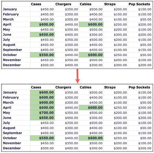
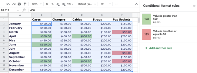
Here, we have our highest values with a green fill color and our lowest with red.
Head back to Format > Conditional Formatting to fire up the sidebar.
You’ll see all rules you’ve set up for that sheet.
Conditional formatting in Google Sheets gives you a terrific way to see the values you want at a glance.
You canmake negative numbers popor try thecolor scale option.