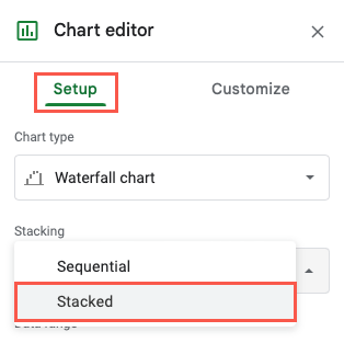
it’s possible for you to then view the data sequentially or stacked for the most effective visual.
We’ll show you how in this guide.
Here, we’ll look at two examples of a waterfall chart in Google Sheets.
What Is a Waterfall Chart?
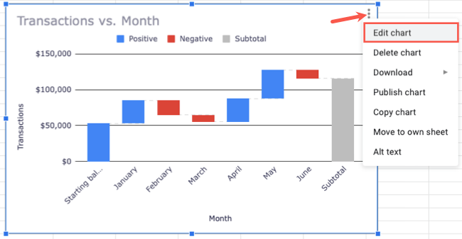
Waterfall charts show how adding or subtracting values affect a starting point over time.
For example, you might chart a checking or savings account with money coming in or going out.
Or, you might track inventory for a product with shipments added and sales subtracted.
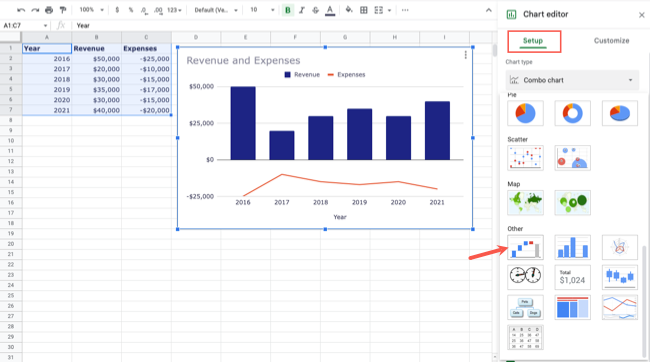
Set Up the Data
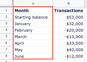
First, you must set up your data correctly.
You should use the first data column to list the headings for each row.
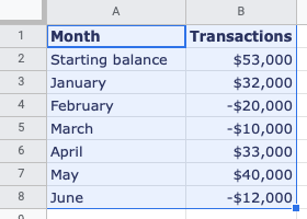
The headings will display on the horizontal axis of the chart.
In the subsequent columns, enter the numeric data corresponding to each row.
Each row is a bar on the waterfall chart.
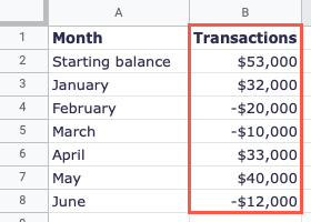
you’re free to do this by dragging your cursor through it.
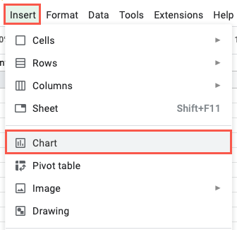
Select Insert > Chart from the menu or nudge the Insert Chart button in the toolbar.
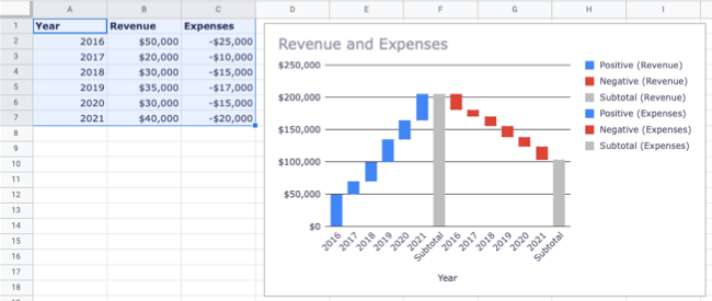
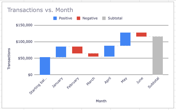
You’ll also notice a Subtotal bar on the far right in gray.
This displays the data from the columns stacked on the same bars rather than separately in sequential order.
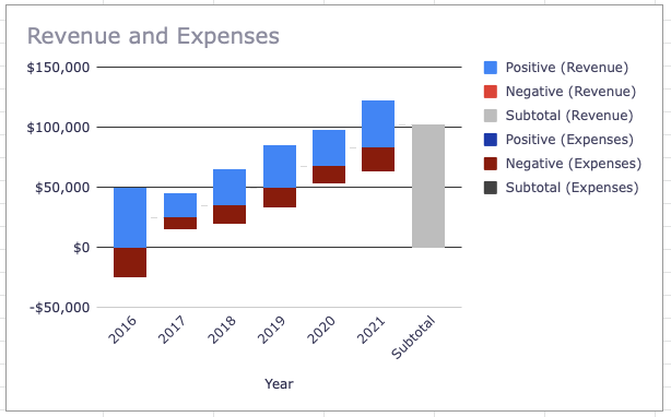
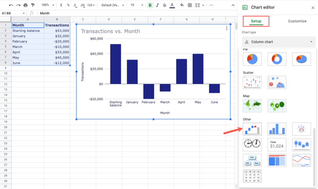
The chart will then update to display the column data on the same bars with different colors.
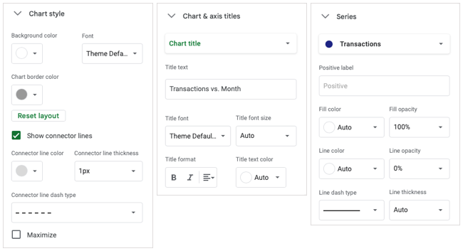
Go to the Customize tab and expand the section you’re gonna wanna update the chart.
Waterfall charts are helpful visuals for showing values that change over time.
For more, check out how tomake a pie chartor how tocreate a line graphin Google Sheets.