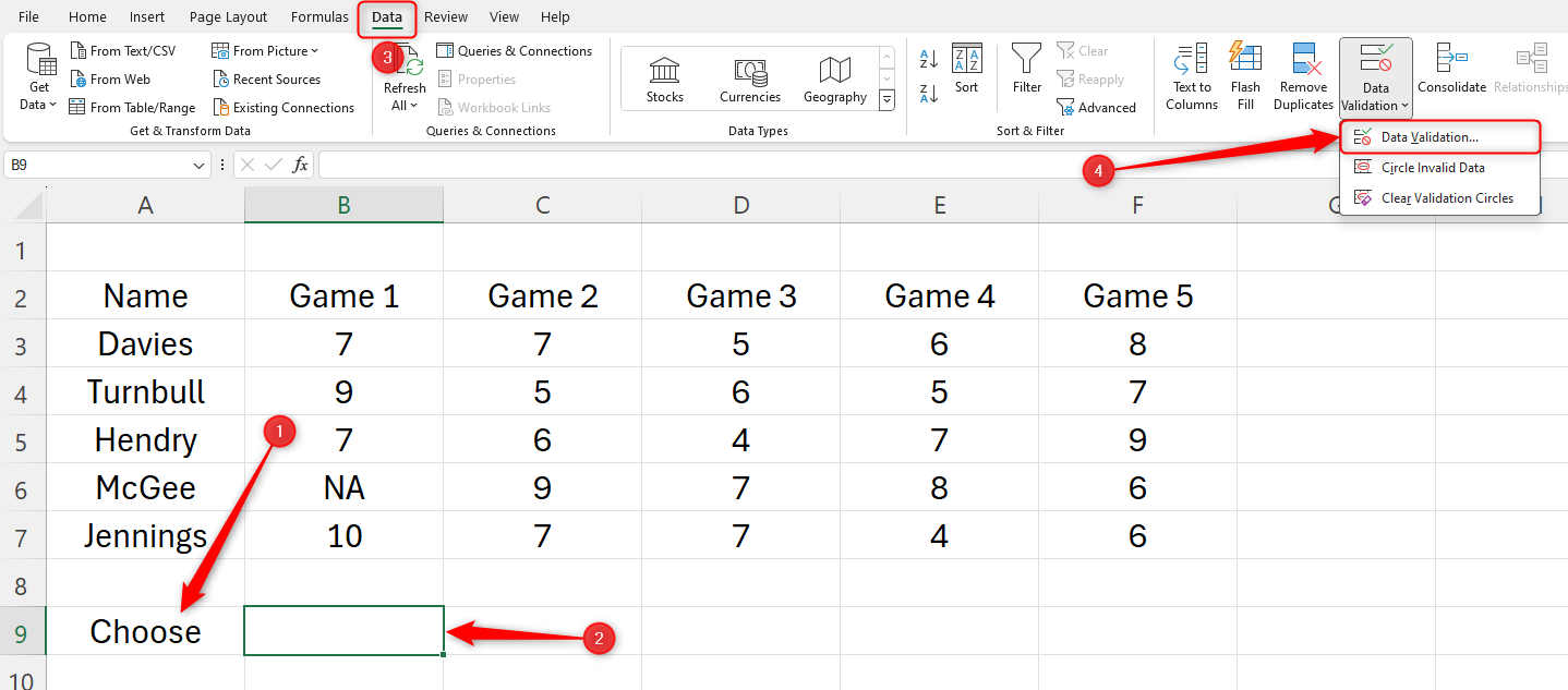
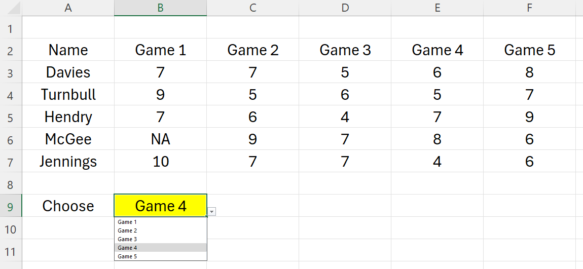
Start by typing an action word in the cell next to where your drop-down will go.
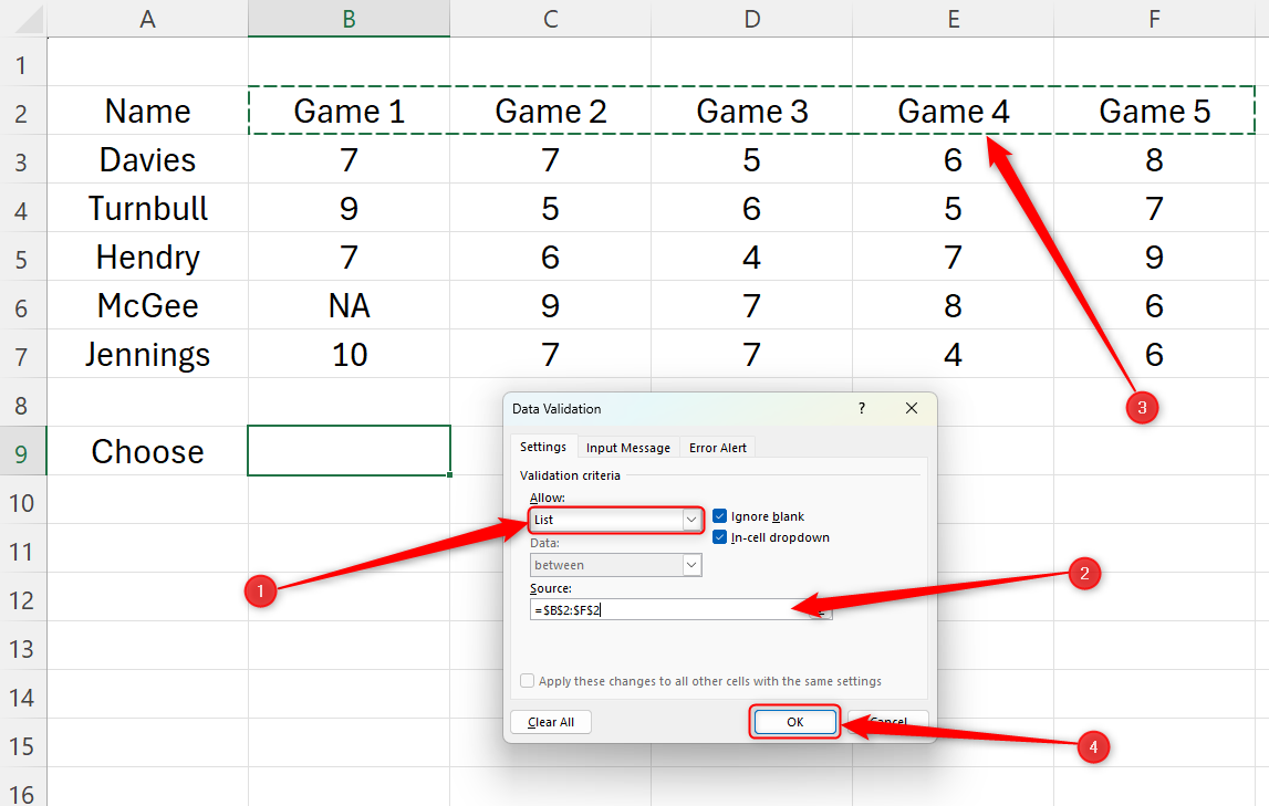
In the Data Validation window, choose “List” under Allow.
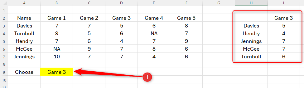
We’ve also formatted our Choose cell to make it stand out.
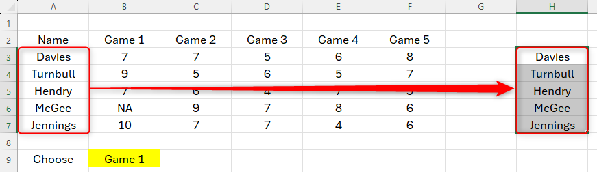
The chart we create later on will be created using the information in this data retrieval table.
From this point, we’ll call the main data tableTable 1, and the data retrieval tableTable 2.
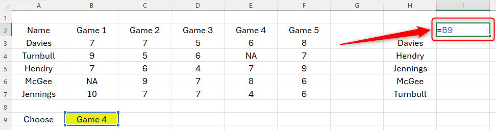
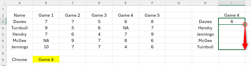
To continue creating Table 2, it’s crucial that you give the next column a heading.
Press Enter to see the column heading in Table 2 adopt the drop-down selection.
Try changing the drop-down selection to see the column heading in Table 2 change.
Otherwise, your formula will not work when you complete the rest of the data in Table 2.
Let’s see this in action.
We now need to initiate the parenthesis and tell Excel where the data is in Table 1.
To do this, highlight all the data in Table 1, butnotthe column and row headings.
Press F4 to make this an absolute reference, and add a comma.
TypeMATCH, open a new parenthesis, and tap the first entry in the first column of Table 2.
In our case, that’s Davies in cell H3.
Next, Excel needs to know what it will use as its reference to look up in Table 1.
And again, we need to tell Excel where to find that data in Table 1.
In our example, that’s cells B2 to F4.
Don’t forget to press F4 after you’ve referenced these cells.
Then, add a comma, a 0, and wrap up the two parentheses together.
Finally, press Enter.
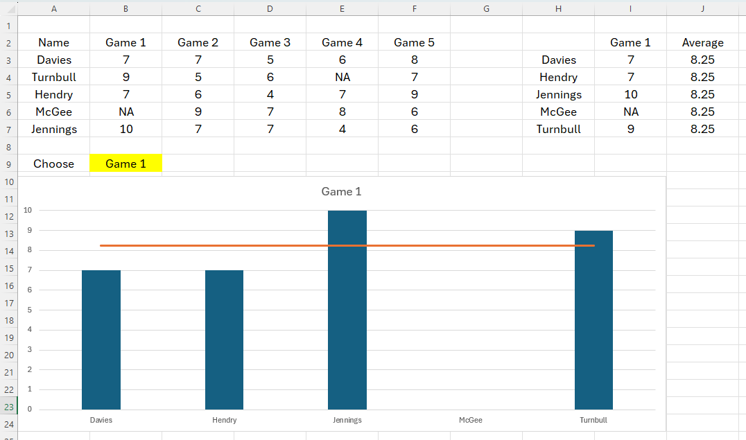
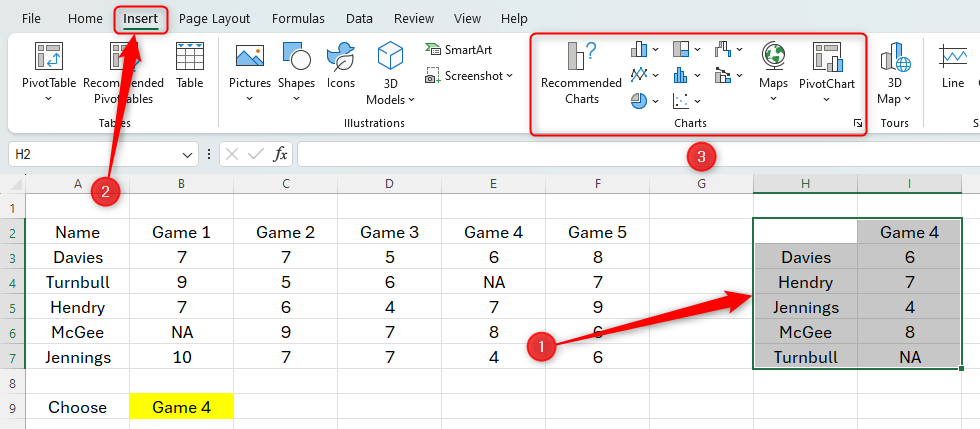
Now that Table 2 successfully changes depending on our drop-down selection, we’re ready to create the chart.
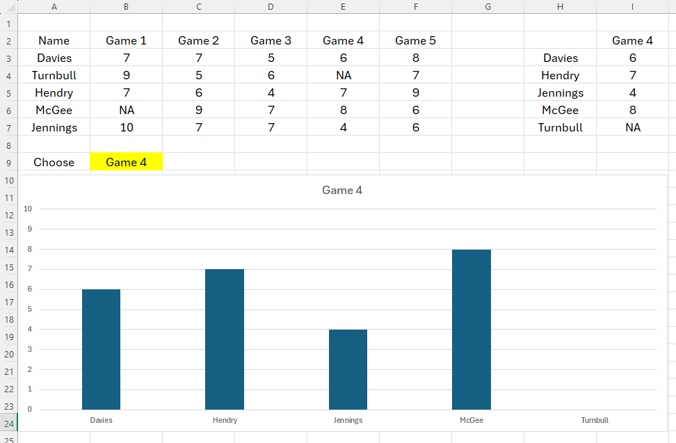
We’ve gone with a simple 2D column chart.
You’ll also see your chart title change.
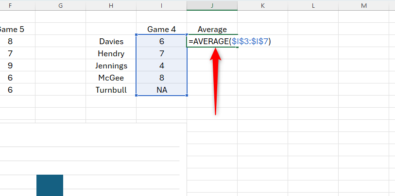
Add another column heading to Table 2, and call itAverage.
Now,use the AVERAGE functionto capture the average of the selected data.
Press F4 to make this an absolute reference, and then shut the parentheses and press Enter.
Then,use the AutoFill handle to click and drag the formula down to the bottom of the column.
We now want to add the average data to our chart.
Click anywhere towards the edge of your chart and click “Chart Design” on the ribbon.
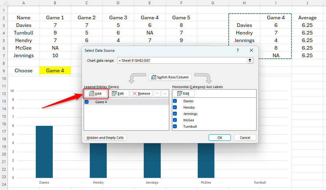
Then, head to the Data group and click “Select Data.”
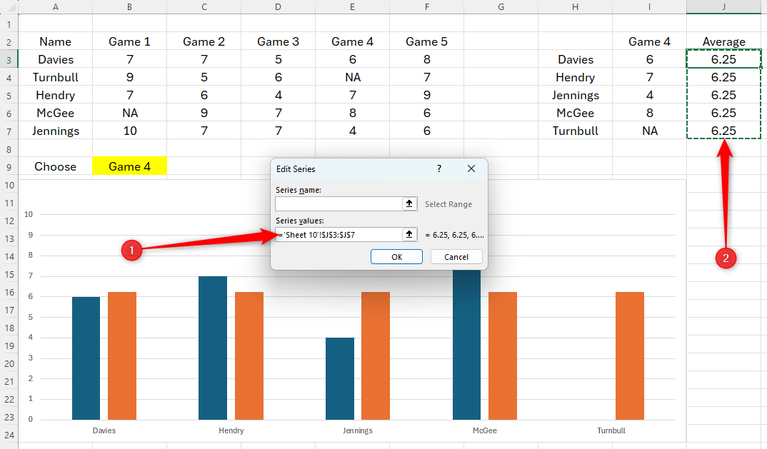
In the Select Data Source window, click “Add.”
Click “OK,” and you will see the average appear as an additional bar in your chart.

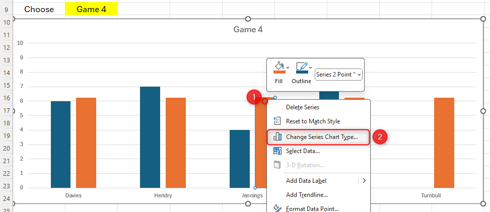
Click OK to see the outcome, and change the drop-down choice to see your chart change dynamically!
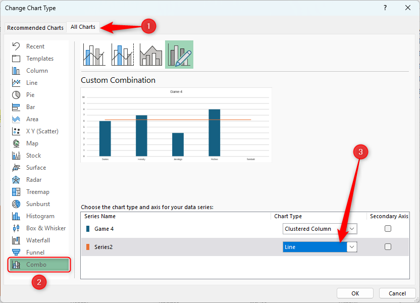
you might then format your line so that it stands out in the way that you want it to.