It’s for an earlier version of Excel, but the interface really hasn’t changed much.
That guide talks about formatting specific cells based on their content.
For example, say you use a spreadsheet to track hours that employees have worked.

But what if you wanted to use a cell’s value to highlight other cells?
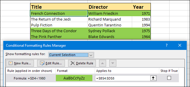
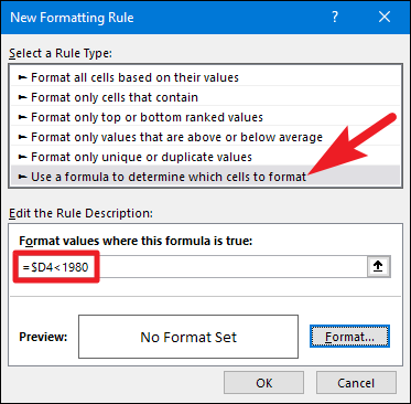
We’re going to use conditional formatting to highlight all the rows with movies made before 1980.
The data doesn’t have to be text-only; you’re able to use formulas freely.

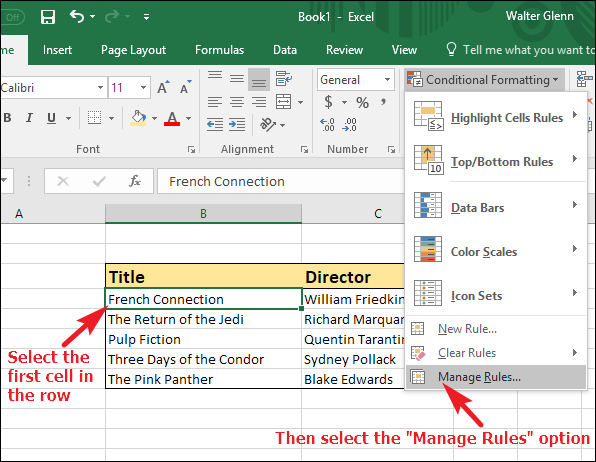
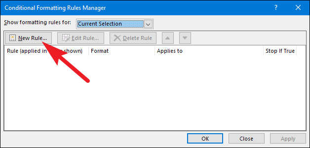
Step Three: Create The Conditional Formatting Rules
Now we come to the meat and potatoes.
If you’re already somewhat familiar with conditional formatting (or just adventurous), let’s forge on.
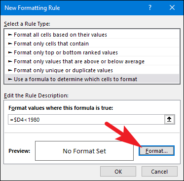
In the “Conditional Formatting Rules Manager” window, smack the “New Rule” button.
This is the trickiest part.
Note the dollar sign before theD.
The<1980part of the formula is the condition that has to be met.
Of course, you could use much more complex formulas if you should probably.
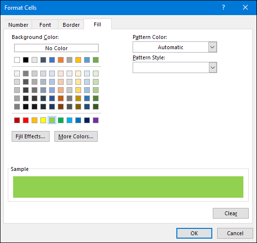
Next, you’ll define the formatting that happens if the formula is true.
In the same “New Formatting Rule” window, hit the “Format” button.
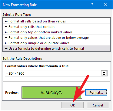
When you’re done applying your formatting, hit the “OK” button.
Back in the “New Formatting Rule” window, you could now see a preview of your cell.
If you’re happy with the way everything looks, smack the “OK” button.
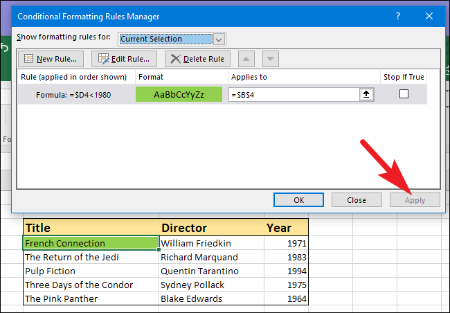
You should now be back to the “Conditional Formatting Rules Manager” window.
If the formatting of your selected cell changes, that means your formula is correct.
Now that you have a working formula, it’s time to apply it across the entire table.
As you might see above, right now the formatting applies only to the cell we started off with.
The “Conditional Formatting Rules Manager” window collapses, giving you access to your spreadsheet.
Drag to resize the current selection across the entire table (except for the headings).
If you have more complex needs, you’re free to create additional formulas.