With conditional formatting in Excel, you’re able to automatically highlight those numbers.
you could choose a column, row, cell range, or non-adjacent cells.
Go to the Home tab and tap the Conditional Formatting drop-down arrow in the Styles section of the ribbon.
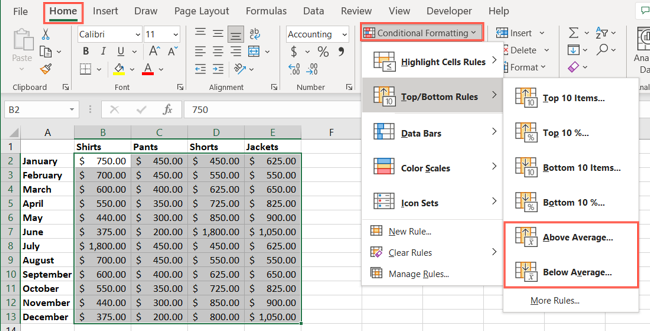
Move your cursor to Top/Bottom Rules and you’ll see Above Average and Below Average in the pop-out menu.
Pick the one you want to use.
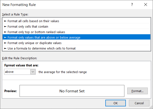
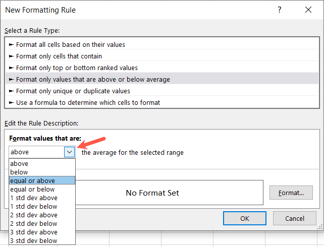
In the pop-up window, you’ll see a few default formats in the drop-down list.
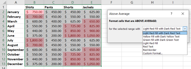
But you may want more detail or different formatting.
By creating a rule from scratch, you’re free to tailor it to fit your needs.
pick the Conditional Formatting drop-down arrow and select “New Rule.”
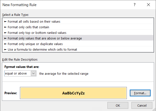
At the top of the pop-up window, choose Format Only Values That Are Above or Below Average.
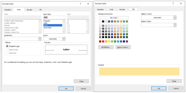
Select “Format” and then choose how you want to highlight those cells.
you’re able to also use a combination of formats if you like.
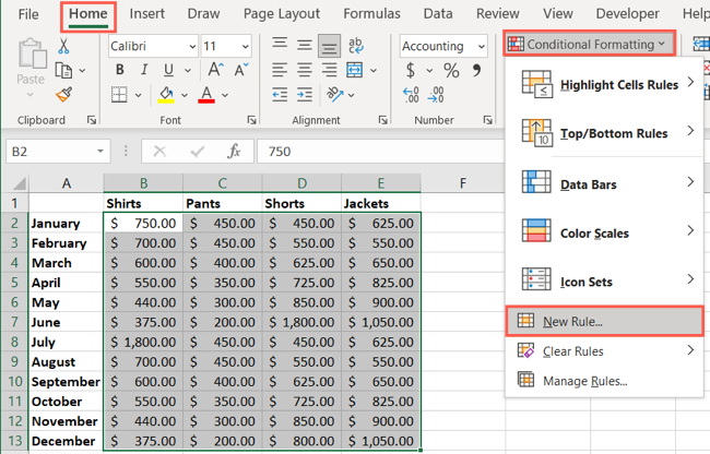
Click “OK” when you finish.
You canapply more than one ruleto the same set of cells if you wish.
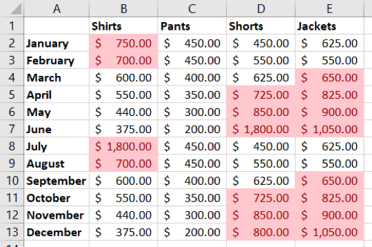
you could use it tohighlight top- or bottom-ranked values, spotcertain dates, or findduplicates in your sheet.