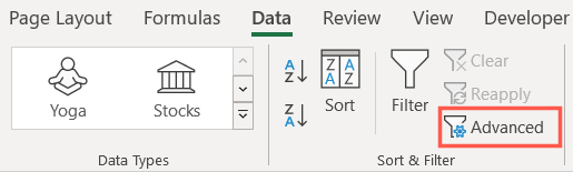
Then, select your data set and kick off the Advanced filter on the Data tab.
Complete the fields, click OK, and see your data a new way.
Here, we’ll explain how to create an advanced filter in Excel.
These should match those for your data as they’ll be used for the filter criteria.
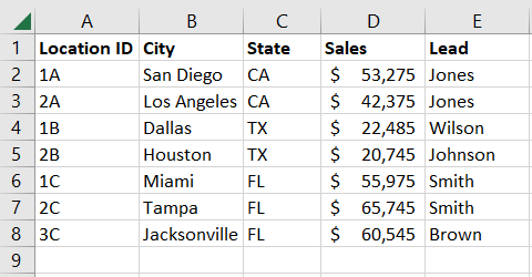
We’ll be using an example throughout this tutorial, so below is the data we’re using.
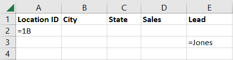
We then insert five rows above our data.
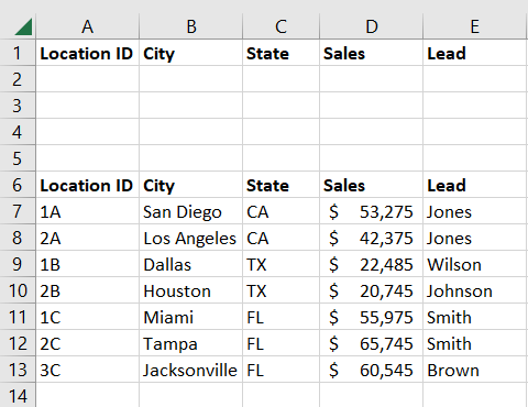
We have one row for labels, three for criteria, and one blank row.
We then copy our column headers into the first row.
You canname your criteria rangeto automatically pop it into the filter if you like.
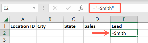
The first equal sign begins the string and the quotations marks contain the criteria.
it’s possible for you to use the normalcomparison operatorsfor your conditions.
Here are a few examples.
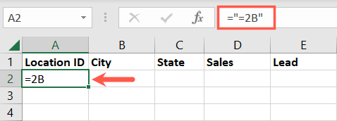
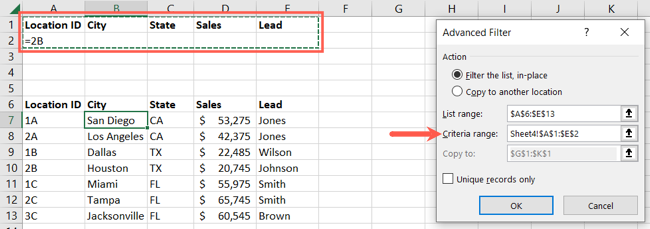
Here, we’ll filter our data based on the Location ID 2B.
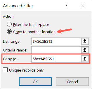
In the pop-up box, start by choosing where you want the filtered data to appear.
you’ve got the option to filter it in place or in another location.
If you choose the latter, enter the location in the Copy To box.
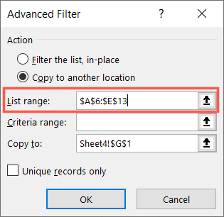
Now confirm the cells in the List Range box.
Excel should have added them for you automatically, so simply see to it they’re correct.
Then, enter the cell range into the Criteria Range box.
Be sure to include the column label cells and only additional rows with cells that contain criteria.
If you includeempty rows, it’s highly likely that your filter results will be incorrect.
Optionally check the boxif you want unique recordsonly.
Click “OK” when you finish.
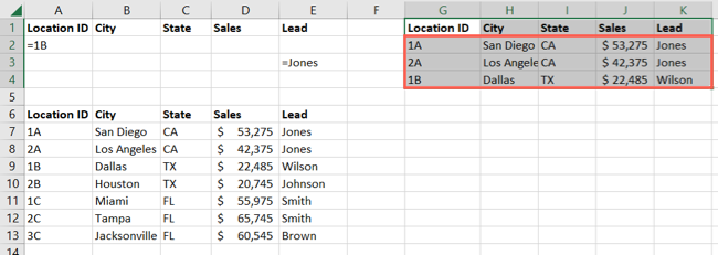
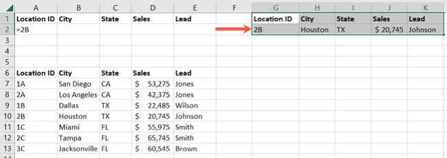
You should then see your filtered data.
If you chose to filter your data in place, the other rows should be hidden.
Here, we picked a location in our sheet for the filtered data.
it’s possible for you to do that with an advanced Excel filter.
As an example, we’ll filter our data for Location ID’s 1B and 2B.
Click “OK” to apply the filter.
You should then see both results from the filter in the location you chose.
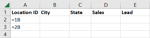
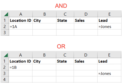
This can beAND or ORcriteria.
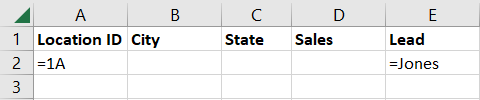
Or you’re able to filter for Location ID equals 1BorLead equals Jones where any conditions are true.
For this filter, we change our criteria range since it only includes rows 1 and 2.
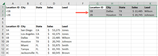
You may see the same thing when reusing the same cell range.
We then have our one result.
Remember that placing the criteria in the same row indicates the AND operator.
For this, you place the conditions in separate rows below the corresponding labels.
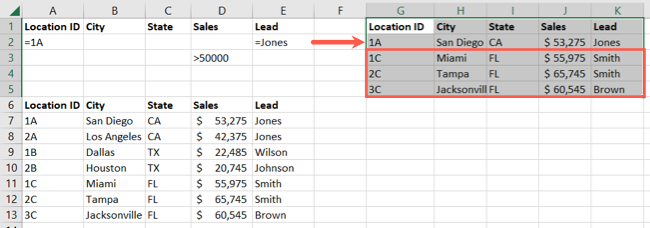
Because we used the OR criteria, any conditions we included were met.
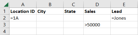
We’ll filter for Location ID equals 1AandLead equals JonesorSales is greater than 50,000.

Here, we have row 2 containing our AND criteria, 1A and Jones.
Then, additional rows 3 through 5 containing our OR criteria for Sales greater than 50,000.
Related:How to Apply a Filter to a Chart in Microsoft Excel