Let’s look into this in more detail.
Excel’s TAKE function only works in Microsoft 365 or Excel for the web.
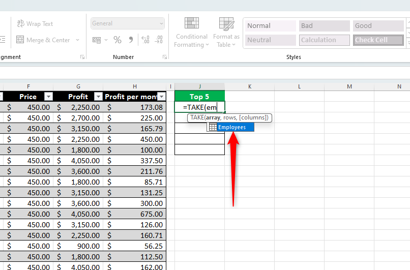
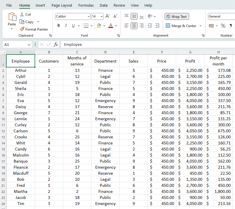
You’re now ready to extract data.
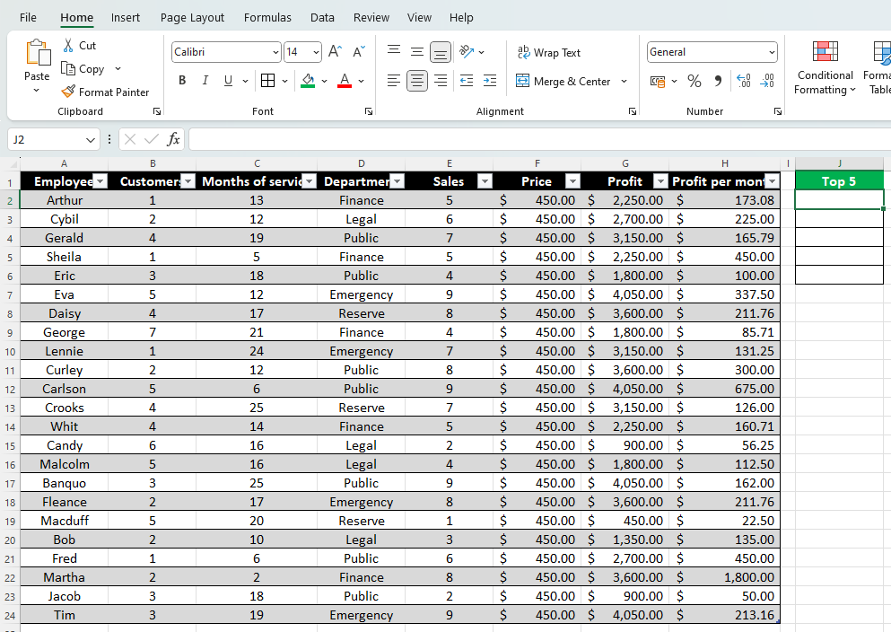
In our case, we’ve chosen cell J2 and the header “Top 5.”
Then, add a comma.
In our case, we want the top five employees.
Therefore, we throw in “5” and add a comma.
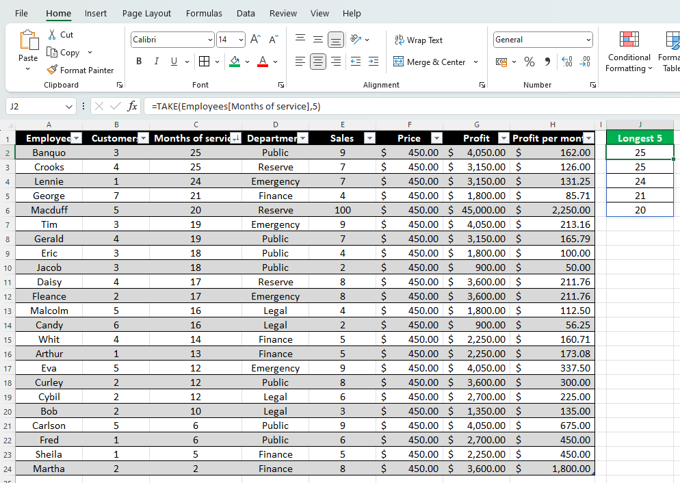
If we wanted the last five rows, we’d key in “-5”.
To extract all rows, simply don’t include the number, and add the comma.
Again, jot down “-” if you want to extract the lastxcolumns.
To extract all columns, miss out the number and press Enter.
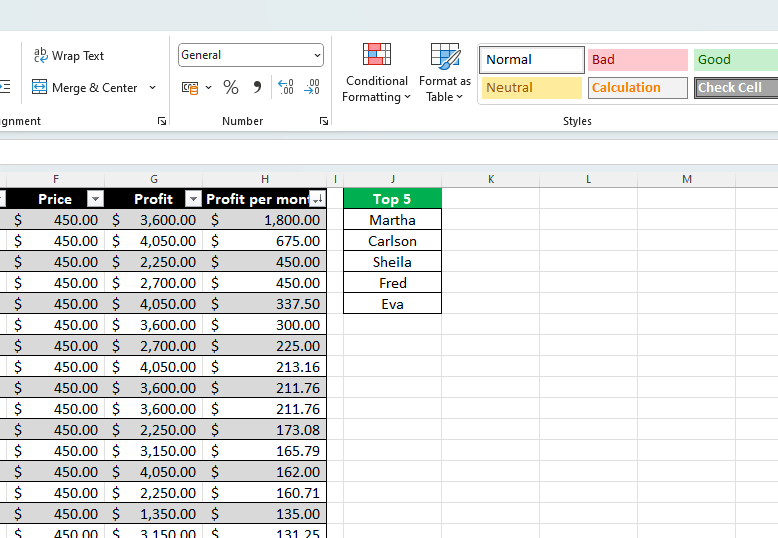
You will now see the desired outcome.
Remember to filter the corresponding column in your table.
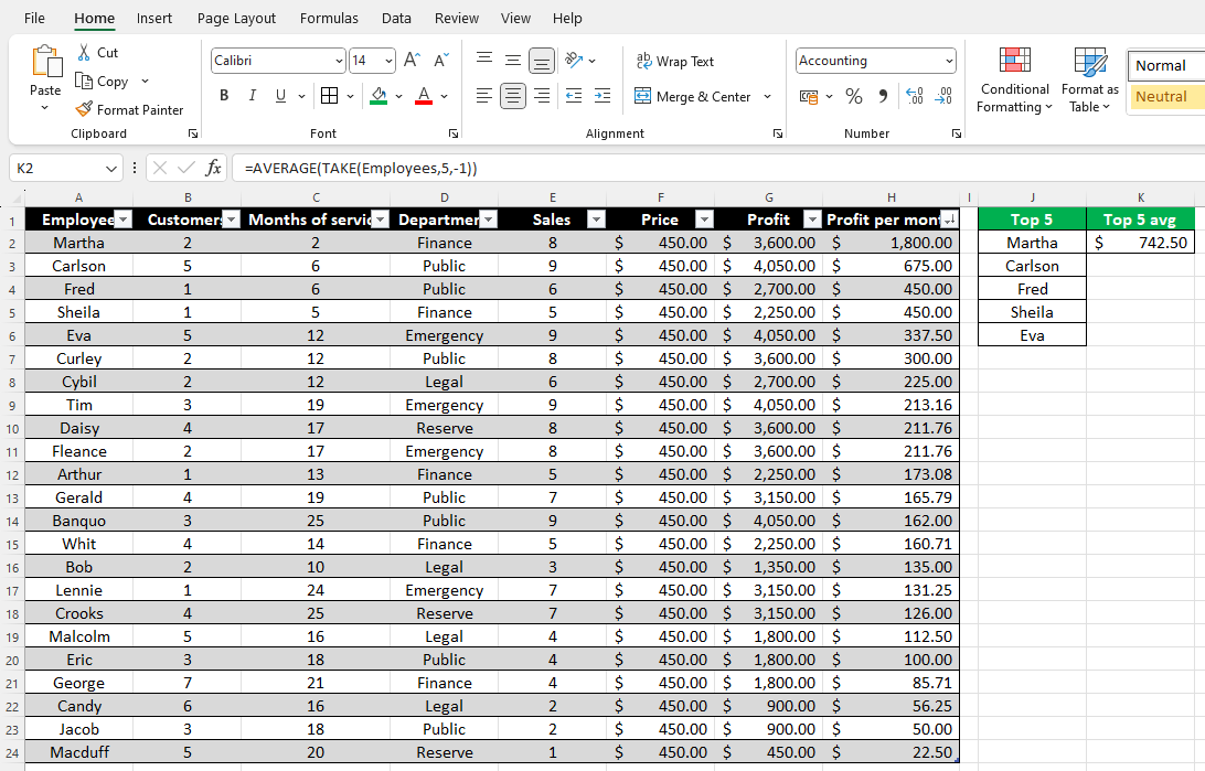
For example, let’s say we want to work out the average earnings of the top five employees.
You now have a fundamental understanding of how the TAKE formula works in Excel.