Here’s how to use it.
Let’s look into this in more detail.
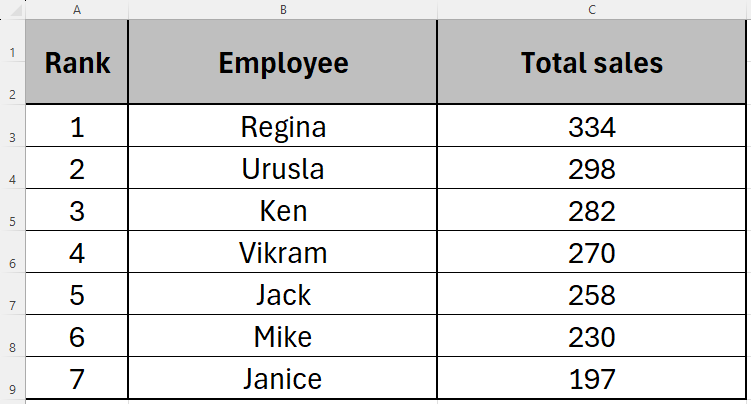
We can use the RANK function toyou guessed itrank the employees based on their total sales.
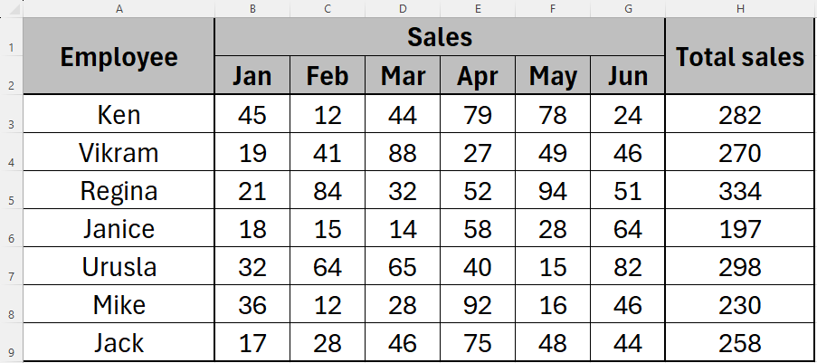
To do this, we need to create a ranking column in our existing table.
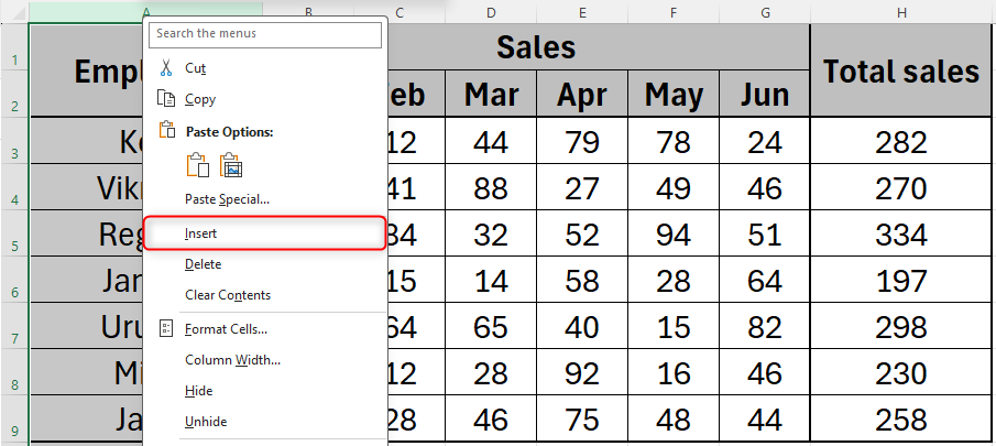
and click “Insert”.
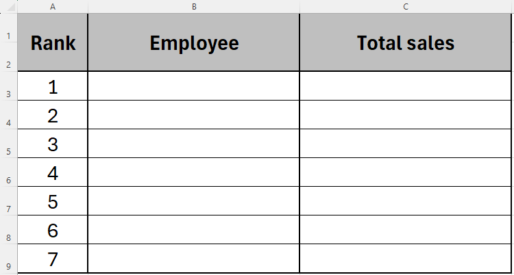
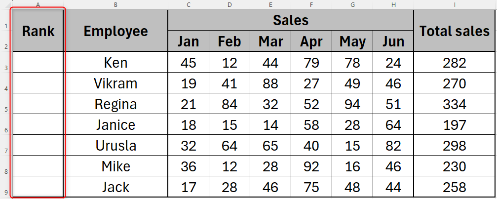
You will then see a new, blank column appear at the left-hand side of your table.
Format this column as you wish and name the column “Rank”.
We’re now ready to begin our RANK formula.
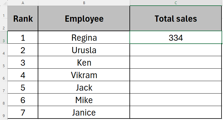
Finally,use Excel’s AutoFill functionto find the rankings for the remaining data in your table.
Your table now clearly tells you where each value ranks within your set of data.
For tidiness, you canrename your worksheet"Totals".
What are RANK.EQ and RANK.AVG?
![]()
They both follow exactly the same syntax and processes as RANK in Excel.
We’re now ready to create the league table.
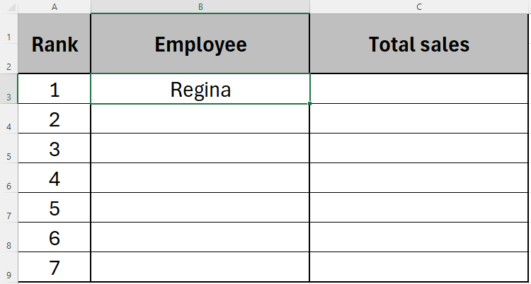
To do this, we need touse Excel’s VLOOKUP function.
![]()
In this case, we’re sourcing data from the Totals sheet in our workbook.
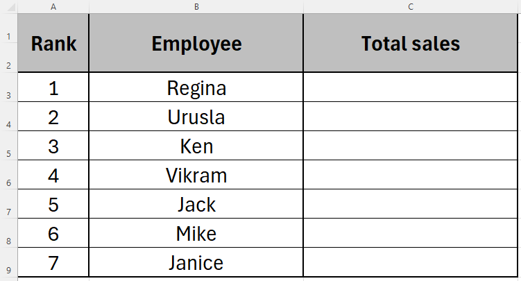
In this example, we want to see the name of the person who ranks first.
Use Excel’s AutoFill function to complete the rest of the employees' names.