And in no scenario is this truer than in its wish to help you visualize data more efficiently.

What Is a Heat Map and What Are They Used For?

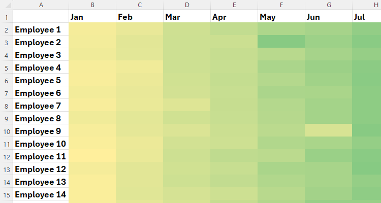
This means you might see trends and anomalies at a glance.

iPhone 16e with iPhone 16 Plus and iPhone 16 Pro in hand against grey wall.

But this Excel tool isn’t exclusively reserved for corporate finances or complicated data analysis.

Let’s explore in more detail how this can be done.

Create Your Data Set

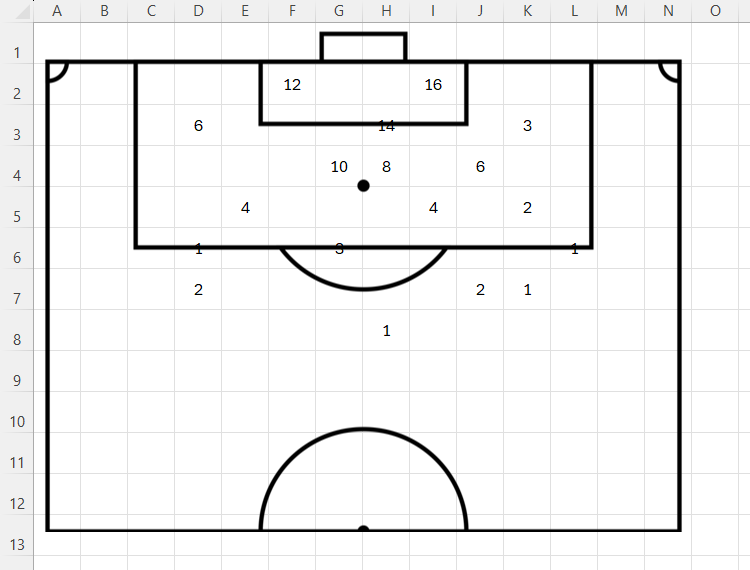
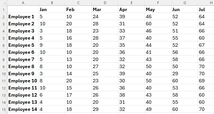
The first step is to create your statistical data in its simplest form.

An Excel table with a named range.

If you wish, you canformat your Excel tableso that it’s easier to add more data later on.

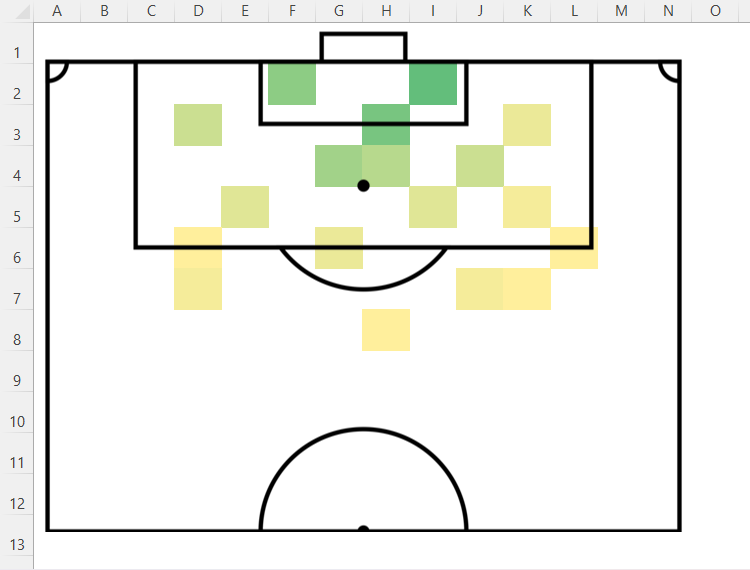
you’re able to do the same with any image outline to create a heat map in Excel.

Apply Conditional Formatting

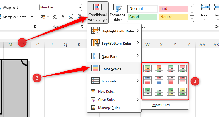
The next step is to apply the color scales to your data.

A heat map in Excel with employees in column A, months in row 1, and the heat map displayed between the two variables.

First, select all the cells that will form the heat map.

Then, hold Shift while using your arrow keys to opt for relevant cells.

In my case, I’ll choose the “Green To Yellow” scale.

A heat map in Excel showing a soccer pitch and certain areas colored according to figures placed in cells.

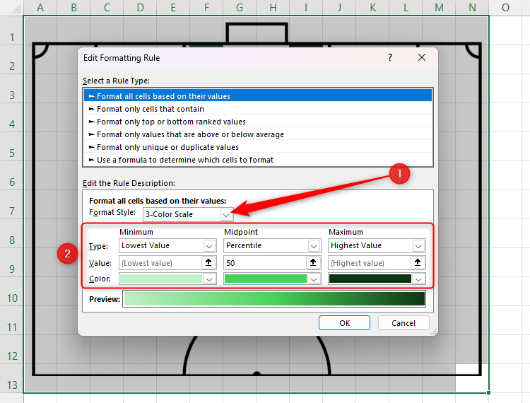
If none of the preset options pique your fancy, click “More Rules” instead.

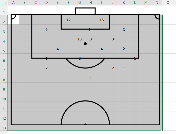
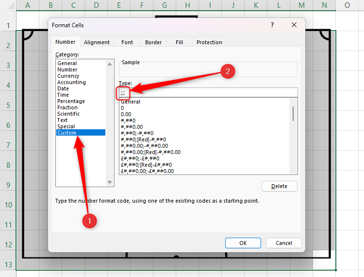
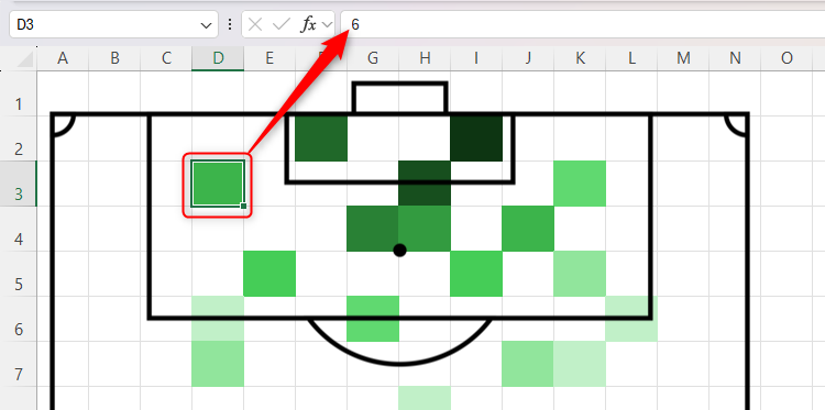
To hide the figures, choose the cells to which you applied the conditional formatting in the previous step.

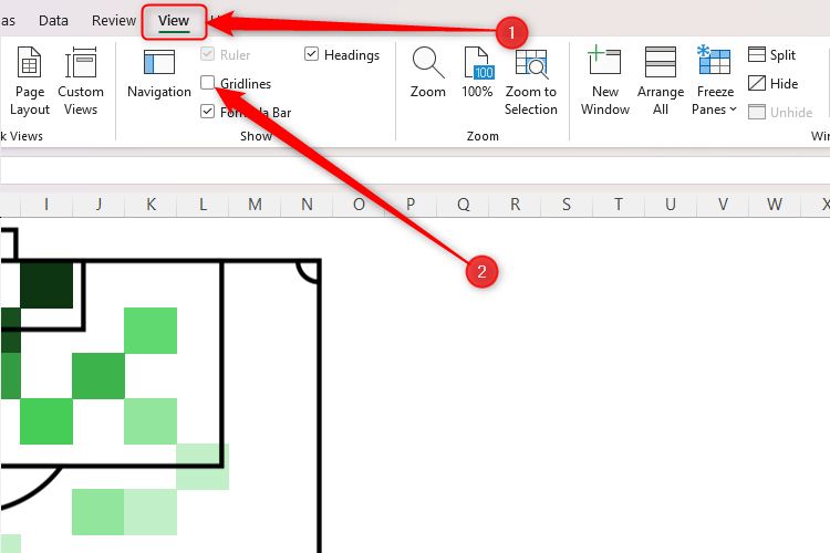
Removing the gridlines is much more straightforward.

An Excel worksheet containing monthly employee data.

In the View tab on the ribbon, uncheck “Gridlines” in the Show group.

An Excel worksheet containing a soccer pitch outline, and numbers inserted into certain cells underneath.

An Excel worksheet containing a soccer pitch outline, and numbers inserted into certain cells underneath. All applicable cells are selected, ready to be formatted.

An Excel sheet containing data, and the Color Scales option in the Conditional Formatting drop-down menu is selected.

An Excel worksheet containing a soccer pitch outline, and numbers inserted into certain cells underneath. The cells are colored using conditional formatting.

The Edit Formatting Rule dialog box in Excel, with the three-color scale selected and the parameters adjusted.

The Format Cells dialog box, with the Number tab opened, the Custom number type selected, and three semicolons typed into the field box.

A cell selected in Excel, with its value showing in the formula bar despite not being displayed in the cell.

The View tab on the ribbon in Excel, with the Gridlines checkbox unchecked.