With that in mind, using conditional formatting can help eliminate these two hurdles.
Conditional formatting formats a cell or a range of cells based on conditions you have applied.
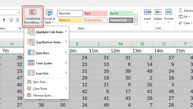
How Do You pull up the Conditional Formatting Tool?

Lucas Gouveia / How-To Geek
From there, you’ll see the many different options available.
I’m not going to run througheveryuse of conditional formatting, as there are hundreds!
This is a really effective way of efficiently cleaning up your spreadsheet.
I use this tool all the time on my vacation packing list.
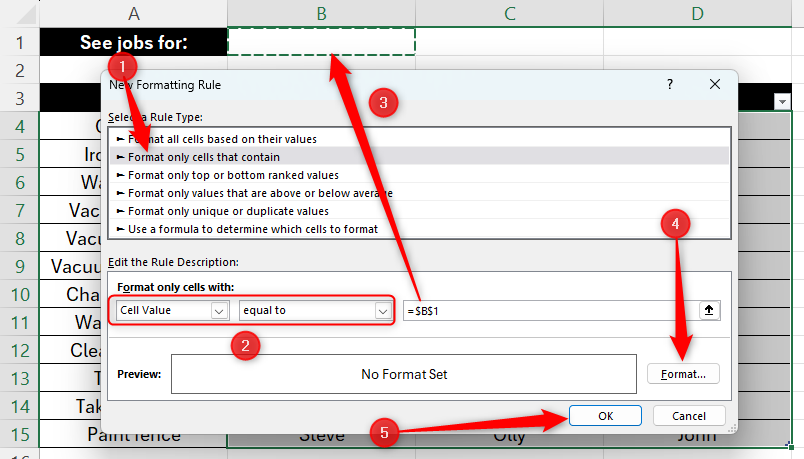
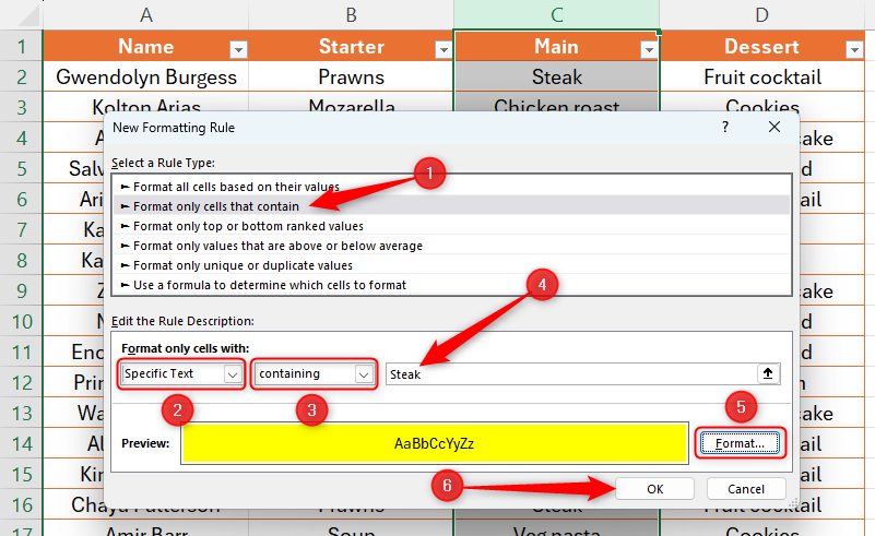
Define the formatting you want for these cells by clicking “Format.”
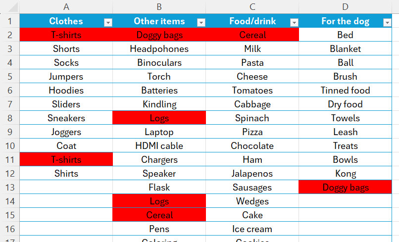
I can now go and delete one of each item that is duplicated.
As a result, I’ll end up with a nice, tidy spreadsheet.
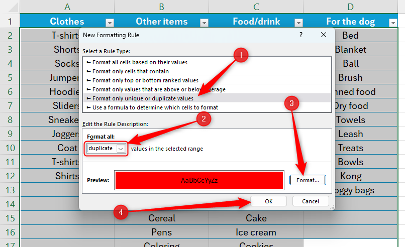
Simply click “Unique” instead of “Duplicate” in the relevant drop-down menu.
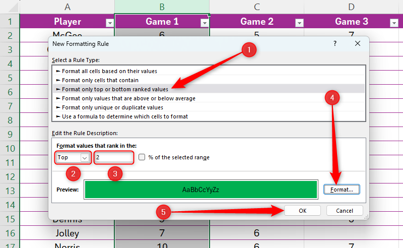
To do this, I make Excelautomatically highlight the highesttwo ratings for each game.
First, opt for data range you want to evaluate.
In my case, it will be the first column containing data.
Then, in the Conditional Formatting menu, click “New Rule.”
Next, in the number field, pop in the parameters of your conditions.
Also check the “%” box if you want to state your parameters as a percentage.
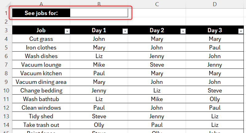
We now want to see all the jobs that a certain family member has been assigned.
To do this, first select all the data you want to search.
Then, in the Conditional Formatting menu, click “New Rule.”
Next, in the second drop-down field, click “Equal To.”

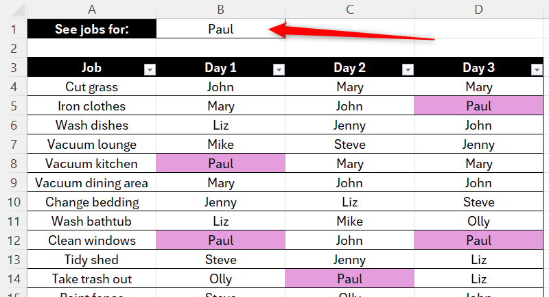
In our case, that’s B1.
You could also choose the variable value from adrop-down list you create in Excel.
However,conditional formatting is equally useful for comparing numbers within a range.
First, go for the data you want to use.
In our case, it’s the ratings from the first game in column B.