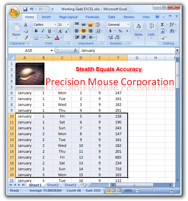
First highlight the data you want to chart on your Excel spreadsheet.
Now that we have the correct data selected we need to click Insert on The Ribbon.
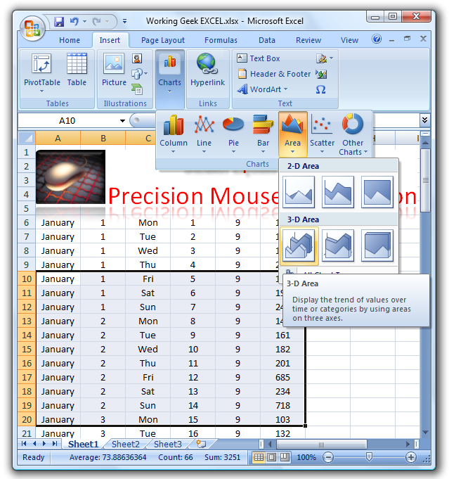
Now select Charts and decide what jot down of chart you want to represent the data.
I usually experiment at this point because you’ve got the option to always undo a certain selection.
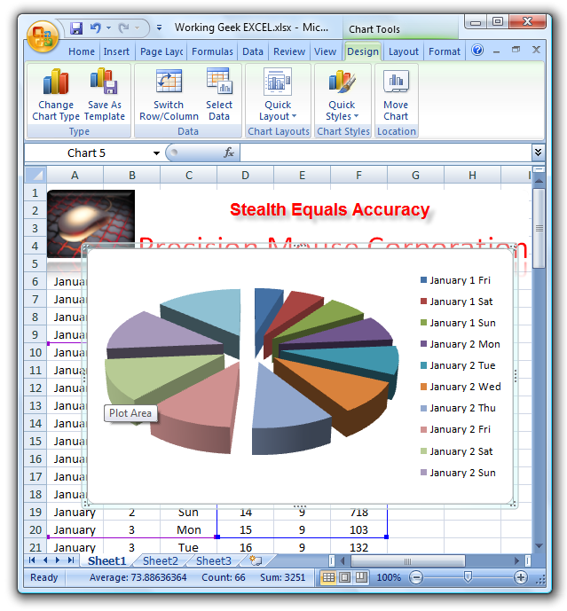
In this example I used the Exploding Pie Chart.
After you make your selection you will get a nice preview of how it looks.
Now we can take this chart and move it anywhere on the Excel document.
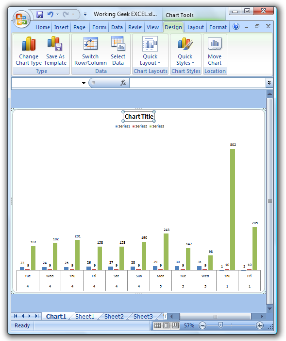
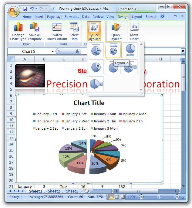
Here we can choose from different types of layouts for the chart.
Again here it’s possible for you to experiment until you get the right fit.
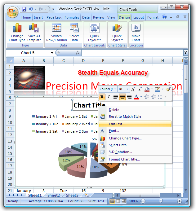
This is the layout I ended up with.
Now lets individualize the chart title by right clicking “Chart Title” and selecting Edit Text.
That is all there is to it!
Later this week I will go over adding details to the chart.