Related
PivotTables are one of the most powerful features of Microsoft Excel.
They allow large amounts of data to be analyzed and summarized in just a few mouse clicks.
Note: This article is written using Excel 2010 (Beta).

A Little History
In the early days of spreadsheet programs, Lotus 1-2-3 ruled the roost.
How did this happen?
What caused such a dramatic reversal of fortunes?

Microsoft, naturally, developed Excel exclusively for Windows.
Secondly, Microsoft developed a feature for Excel that Lotus didn’t provide in 1-2-3, namely PivotTables.
Understanding PivotTables
So what is a PivotTable, exactly?
But unlike a manually created summary, Excel PivotTables are interactive.
There’s a lot more that can be done, too.
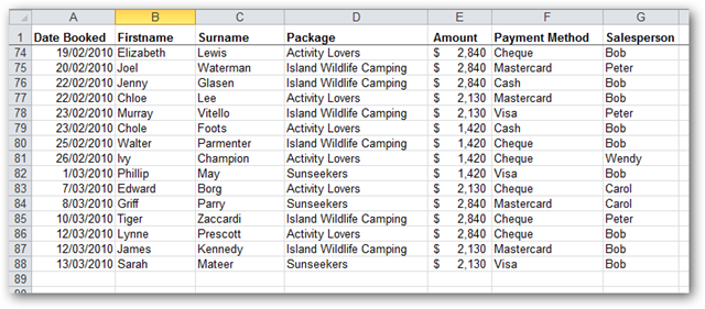
Rather than venture to describe all the features of PivotTables, we’ll simply demonstrate them… An example of this might be the list of sales transactions in a company for the past six months.
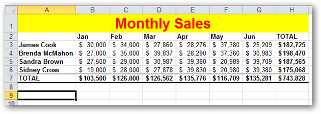
Examine the data shown below:
Notice that this is not raw data.
In fact, it is already a summary of some sort.
So where is the raw data?
How did we arrive at the figure of $30,000?
Where is the original list of sales transactions that this figure was generated from?
How long do you suppose this took?
Most probably, yes.
You see, the spreadsheet above is actuallynota PivotTable.
Let’s find out how… We can do this - and a lot more too!
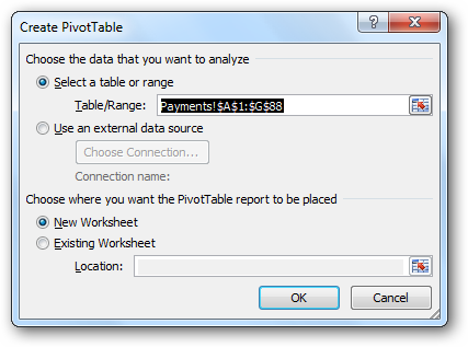
How to Create a PivotTable
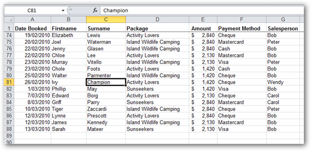
First, ensure that you have some raw data in a worksheet in Excel.
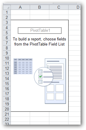
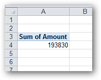
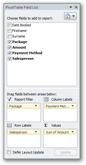
So far, there is nothing in those boxes, so the PivotTable is blank.
A PivotTable is then automatically created to match our instructions.
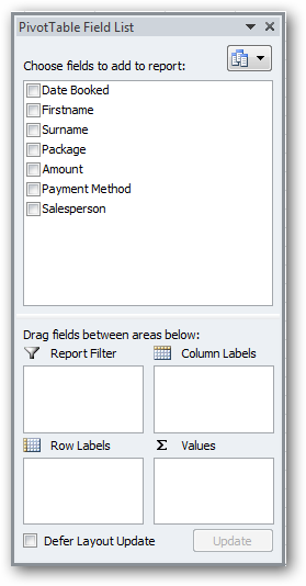
TheValuesbox is arguably the most important of the four.
It is almost always numerical data.
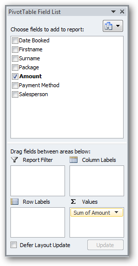
A perfect candidate for this box in our sample data is the “Amount” field/column.
Handy, but not particularly impressive.
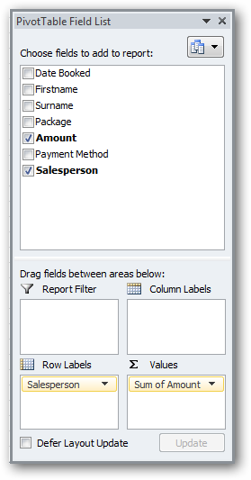
It’s likely that we need a little more insight into our data than that.
So what else can we do?
Well, in one sense our PivotTable is complete.
We’ve created a useful summary of our source data.
The important stuff is already learned!
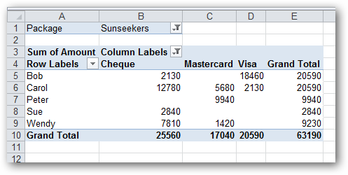
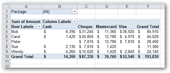
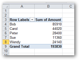
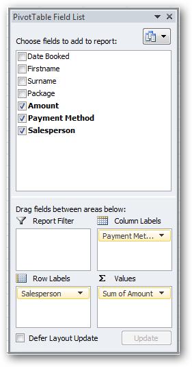
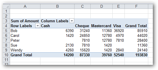
First, we can create a two-dimensional table.
Let’s do that by using “Payment Method” as a column heading.
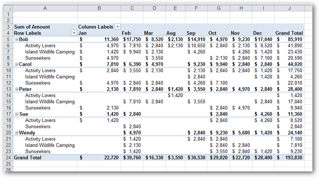
Let’s make it a three-dimensional table.
What could such a table possibly look like?
Well, let’s see…
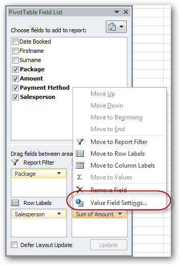
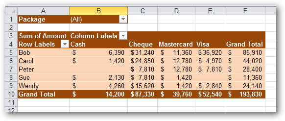
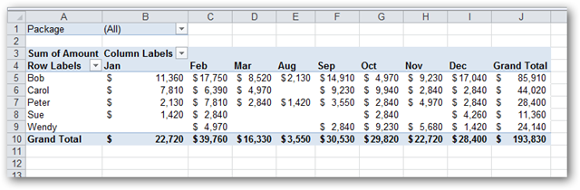
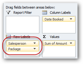
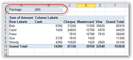
Drag the “Package” column/heading to theReport Filterbox:
Notice where it ends up….
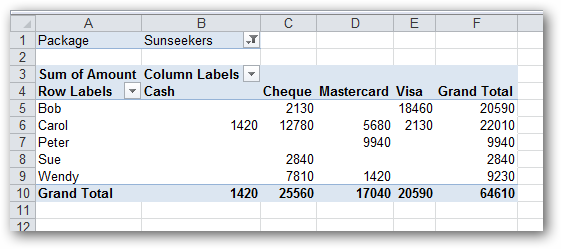
This allows us to filter our report based on which “holiday package” was being purchased.
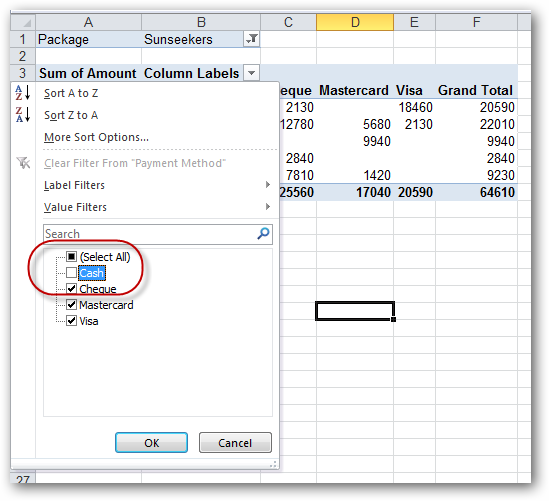
Let’s keep customizing… no cash transactions), then we can deselect the “Cash” item from the column headings.
Formatting
This is obviously a very powerful system, but so far the results look very plain and boring.
Let’s rectify that.
We need a way that will make them (semi-)permanent.
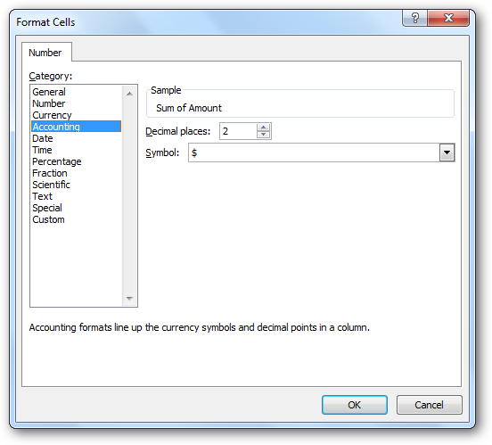
First, we locate the “Sum of Amount” entry in theValuesbox, and hit it.
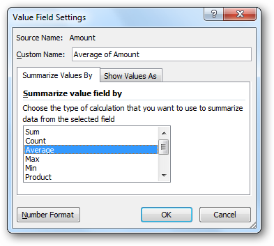
We selectValue Field tweaks…from the menu:
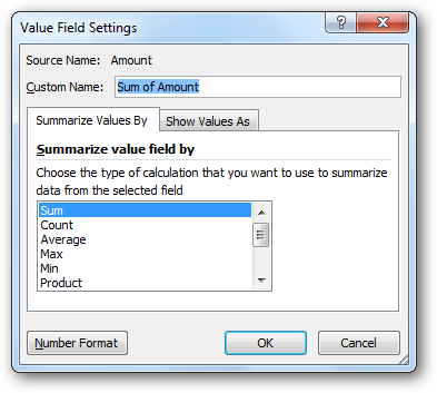
TheValue Field Settingsbox appears.
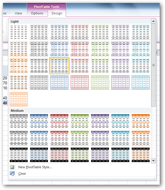
While we’re on the subject of formatting, let’s format the entire PivotTable.
There are a few ways to do this.
Let’s see how this is done.
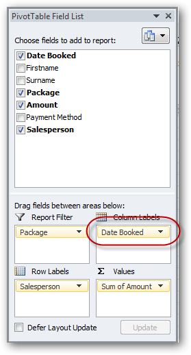
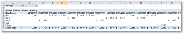
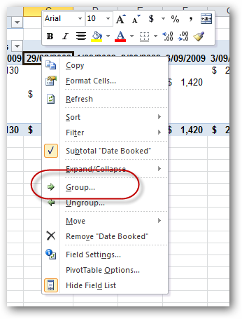
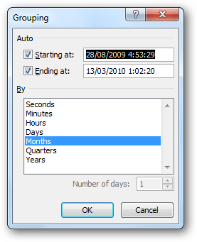
To fix this, right-choose any date and selectGroup…from the context-menu:
The grouping box appears.
We selectMonthsand click OK:
Voila!
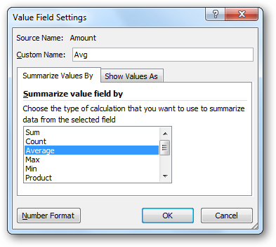
Keeping things simple again, let’s see how to plot averaged values, rather than summed values.
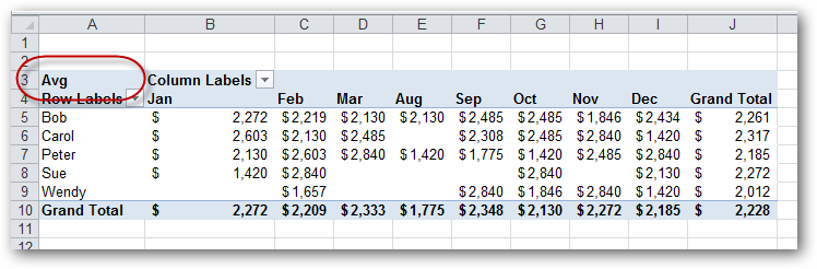
punch in in something like “Avg”:
ClickOK, and see what it looks like.
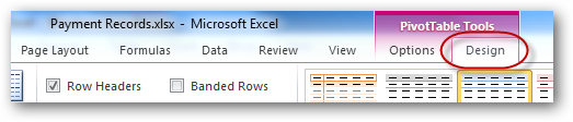
There are also the two ribbon-tabs:PivotTable Tools/OptionsandDesign.
It should work with all versions of Excel from 97 onwards.
Download Our Practice Excel Workbook