Picture thisyour manager has asked you for this year’s key figures.

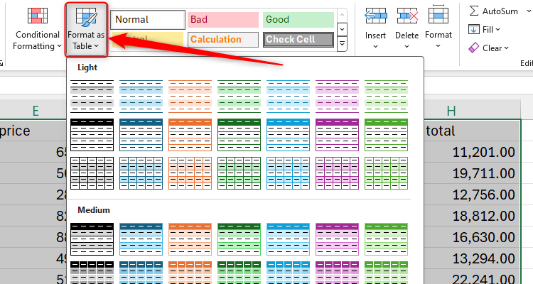
At the same time, think about how you want to display each data set.

Will you use pie charts or line graphs?

Excel project dashboard on a laptop.

Lucas Gouveia / How-To Geek |selinofoto/ Shutterstock

Would a scatter graph or a pie chart work better for some of your data?

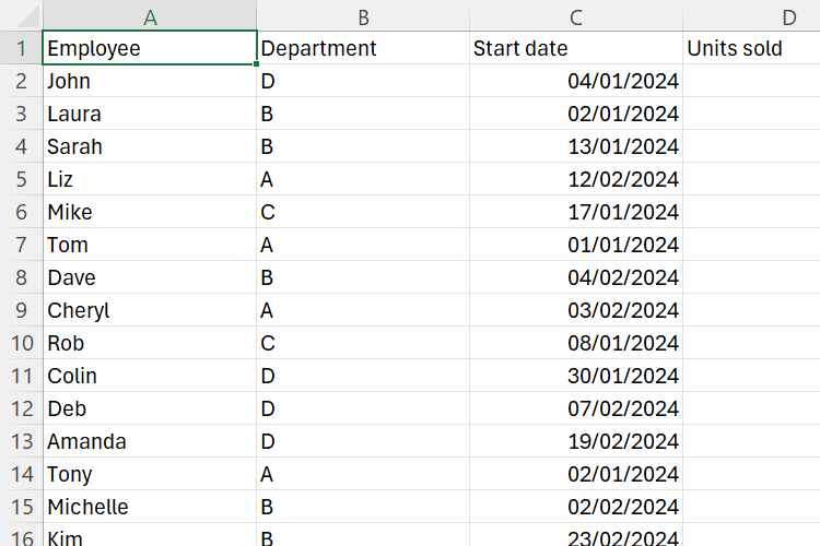
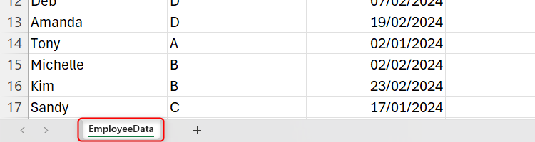
ensure you havegiven each sheet an appropriate name.

verify you also remove any blank rows in your tables.

An Excel sheet containing an unformatted table of employee data.

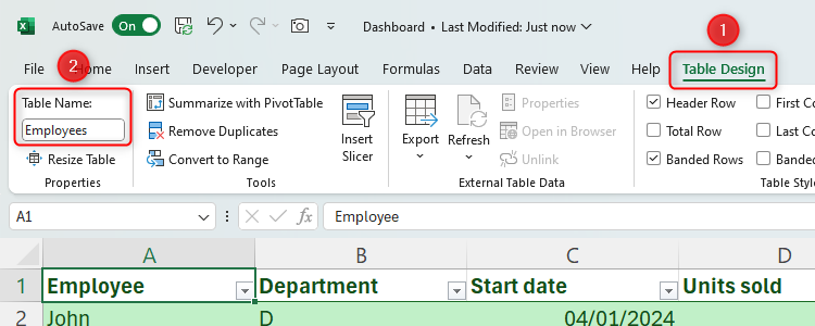
The next step in preparing your data is toname the table.

attempt to keep this to one word, if possible, for easier use later on.

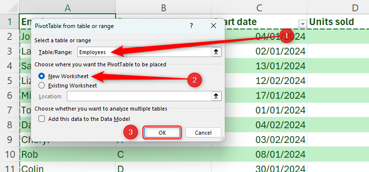
The final prep step is to create a dashboard tab.

An Excel worksheet with a tab renamed ‘EmployeeData.'

hit the “+” symbol next to your tabs and rename itDashboard.

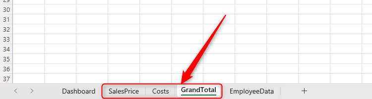
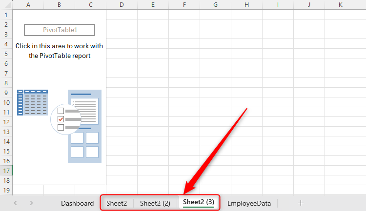
So, you want a separate PivotTable tab for each chart you will create.

We want three charts on our dashboard, so we’ll do this twice.

An unformatted Excel table with the Format As Table button highlighted and the options showing.

after you grab the correct number of PivotTables, rename the tabs according to the data they will contain.

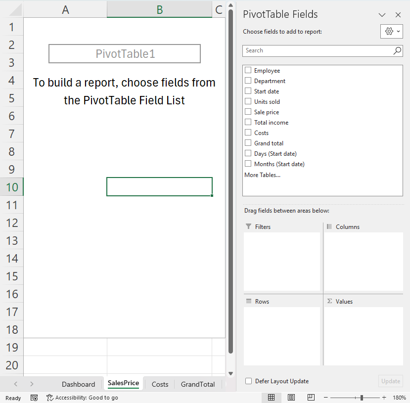
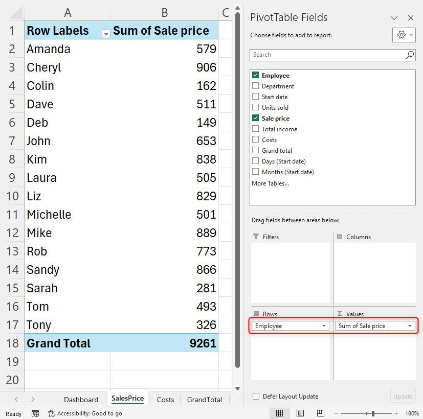
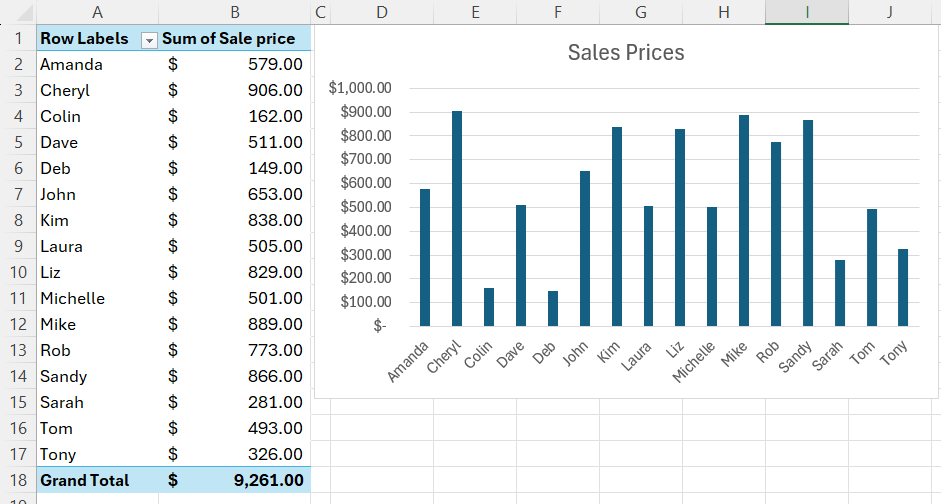
You will see your PivotTable update on the left as you do this.

Step 4: Create Your First Chart

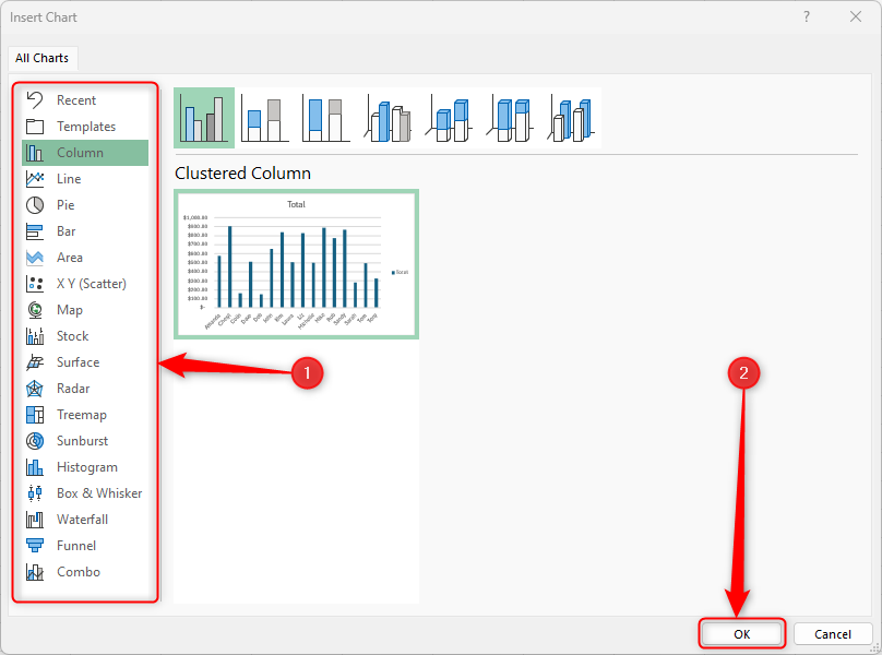
You’re now ready to create your first chart.

An Excel table with the Table Name area in the Table Design tab highlighted. The word ‘Employees’ has been typed into the Table Name box.

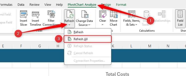
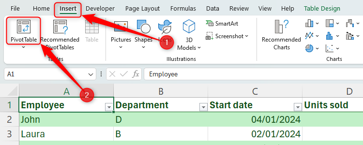
Click anywhere in your PivotTable and head to the ribbon.

In the PivotTable Analyze tab, click “PivotChart.”

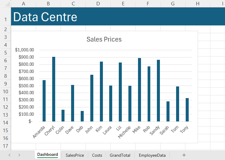
You could even add a stylish header to your dashboard tab.

An Excel workbook with a new tab called ‘Dashboard.’ The ‘+’ symbol is highlighted to demonstrate where to click to add a new sheet.

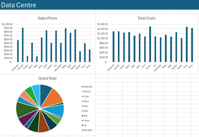
Step 5: Repeat the Process!

Now that you have your first PivotTable and PivotChart, follow the same steps to complete your dashboard.

When repositioning your charts, hold down the Alt key to make them snap into a given position.

An Excel worksheet with the Insert option on the ribbon and the Pivot Table button highlighted.

This is great for lining items up when you have more than one on a worksheet.
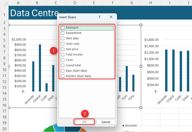
Step 6: Add Slicers

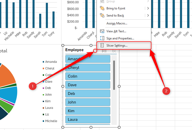
To make your charts more interactive,add slicers.

Click any of your charts, and in the PivotChart Analyze tab, click “Insert Slicer.”

Excel’s PivotTable dialog box, with the name of the table inserted into the Range field, the New Worksheet radio button checked, and the OK button highlighted.

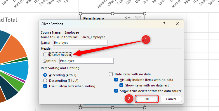
Change the controls according to what you want the slicer to show.

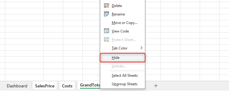
Then,hide your PivotTable tabs, as they could confuse other people when they open your workbook.

To do this, click one of the tabs, hold Ctrl, and then poke the other tabs.

An Excel workbook with three new sheets, all of which contain a PivotTable area.

Then, right-click one of the selected tabs and click “Hide.”

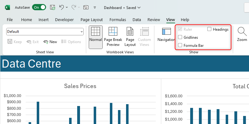
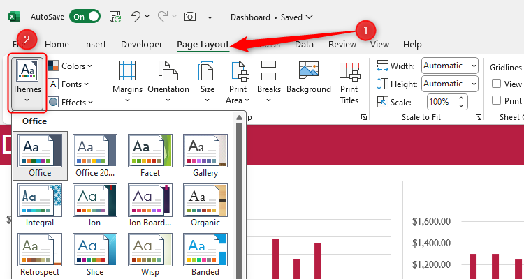
Then, choose a color scheme to make all your charts and layouts match each other.

An Excel workbook with the three sheets containing PivotTables renamed according to the data they will show.

An Excel PivotTable area on the left and the PivotTable sidebar on the right.

An Excel PivotTable sidebar on the right, with ‘Employee’ in the Rows Section and ‘Sum Of Sale Price’ in the Values section.

Excel’s Insert Dialog box with the different types of charts highlighted on the left and the OK button highlighted at the bottom.

A formatted PivotChart in Excel next to the PivotTable used to create it.

An Excel dashboard tab containing a chart.

A dashboard in Excel containing three PivotCharts.

The Insert Slicers dialog box in Excel, with the options highlighted and the OK button selected.

The Slicer Settings option, accessible by right-clicking on a slicer in Excel.

Excel’s Slicer Settings dialog box, with ‘Display Header’ unchecked, and the OK button highlighted.

The slicer’s Report Connections dialog box in Excel, with all PivotTables selected.

The ‘Refresh All’ option in the PivotChart Analyze tab is selected.

An Excel worksheet with the Gridlines, Formula Bar, and Headings options unchecked.

Three tabs in Excel are selected and the ‘Hide’ option, accessible by right-clicking one of the selected tabs, is highlighted.

The Theme menu in Excel, accessed through the Page Layout tab.